[Updated: Sun, Nov 27, 2022 - 14:05:46 ]
Regularization
Regularization is a general strategy to incorporate additional penalty terms into the model fitting process and is used not just for regression but a variety of other models. The idea behind the regularization is to constrain the size of regression coefficients to reduce their sampling variation and, hence, reduce the variance of model predictions. These constraints are typically incorporated into the loss function to be optimized. There are two commonly used regularization strategies: ridge penalty and lasso penalty. In addition, there is also elastic net, a mixture of these two strategies.
Ridge Regression
Ridge Penalty
Remember that we formulated the loss function for the linear
regression as the sum of squared residuals across all observations. For
ridge regression, we add a penalty term to this loss function, which is
a function of all the regression coefficients in the model. Assuming
that there are P regression coefficients in the model, the penalty term
for the ridge regression would be λP∑i=1β2p,
Loss=N∑i=1ϵ2(i)+λP∑p=1β2p,
Loss=SSR+λP∑i=1β2p.
Let’s consider the same example from the previous class. Suppose we fit a simple linear regression model such that the readability score is the outcome (Y) and the Feature 220 is the predictor(X). Our regression model is
Y=β0+β1X+ϵ,
let’s assume the set of coefficients are {β0,β1} = {-1.5,2}, so my model
is Y=−1.5+2X+ϵ.
readability_sub <- read.csv('./data/readability_sub.csv',header=TRUE)

d <-  readability_sub[,c('V220','target')]

b0 = -1.5
b1 = 2

d$predicted <- b0 + b1*d$V220
d$error     <- d$target - d$predicted

d
V220 target predicted error
1 -0.13908258 -2.06282395 -1.7781652 -0.28465879
2 0.21764143 0.58258607 -1.0647171 1.64730321
3 0.05812133 -1.65313060 -1.3837573 -0.26937327
4 0.02526429 -0.87390681 -1.4494714 0.57556460
5 0.22430885 -1.74049148 -1.0513823 -0.68910918
6 -0.07795373 -3.63993555 -1.6559075 -1.98402809
7 0.43400714 -0.62284268 -0.6319857 0.00914304
8 -0.24364550 -0.34426981 -1.9872910 1.64302120
9 0.15893717 -1.12298826 -1.1821257 0.05913740
10 0.14496475 -0.99857142 -1.2100705 0.21149908
11 0.34222975 -0.87656742 -0.8155405 -0.06102693
12 0.25219145 -0.03304643 -0.9956171 0.96257066
13 0.03532625 -0.49529863 -1.4293475 0.93404886
14 0.36410633 0.12453660 -0.7717873 0.89632394
15 0.29988593 0.09678258 -0.9002281 0.99701073
16 0.19837037 0.38422270 -1.1032593 1.48748196
17 0.07807041 -0.58143038 -1.3438592 0.76242880
18 0.07935690 -0.34324576 -1.3412862 0.99804044
19 0.57000953 -0.39054205 -0.3599809 -0.03056111
20 0.34523284 -0.67548411 -0.8095343 0.13405021lambda = 0.2
loss <- sum((d$error)^2) + lambda*(b0^2 + b1^2)
loss [1] 19.01657Notice that when λ is equal to zero, the loss function is identical to SSR; therefore, it becomes a linear regression with no regularization. As the value of λ increases, the degree of penalty linearly increases. The λ can technically take any positive value between 0 and ∞.
As we did in the previous lecture, imagine that we computed the loss function with the ridge penalty term for every possible combination of the intercept (β0) and the slope (β1). Let’s say the plausible range for the intercept is from -10 to 10 and the plausible range for the slope is from -2 to 2. Now, we also have to think of different values of λ because the surface we try to minimize is dependent on the value λ and different values of λ yield different estimates of β0 and β1.
Model Estimation
Matrix Solution
The matrix solution we learned before for regression without regularization can also be applied to estimate the coefficients from ridge regression given the λ value. Given that
- Y is an N x 1 column vector of observed values for the outcome variable,
- X is an N x (P+1) design matrix for the set of predictor variables, including an intercept term,
- β is an (P+1) x 1 column vector of regression coefficients,
- I is a (P+1) x (P+1) identity matrix,
- and λ is a positive real-valued number,
the ridge regression coefficients can be estimated using the following matrix operation.
ˆβ=(XTX+λI)−1XTY
Y(i)=β0+β1X1(i)+β2X2(i)+ϵ(i).
Y <-  as.matrix(readability_sub$target)
X <-  as.matrix(cbind(1,readability_sub$V220,readability_sub$V166))

lambda <- 0.5

beta <- solve(t(X)%*%X + lambda*diag(ncol(X)))%*%t(X)%*%Y

beta
[,1]
[1,] -0.9151087
[2,] 1.1691920
[3,] -0.2206188If we change the value of λ to 2, we will get different estimates for the regression coefficients.
Y <-  as.matrix(readability_sub$target)
X <-  as.matrix(cbind(1,readability_sub$V220,readability_sub$V166))

lambda <- 2

beta <- solve(t(X)%*%X + lambda*diag(ncol(X)))%*%t(X)%*%Y

beta
[,1]
[1,] -0.7550986
[2,] 0.4685138
[3,] -0.1152953We can manipulate the value of λ from 0 to 100 with increments of .1 and calculate the regression coefficients. Note the regression coefficients will shrink toward zero but will never be exactly equal to zero in ridge regression.
Y <-  as.matrix(readability_sub$target)
X <-  as.matrix(cbind(1,readability_sub$V220,readability_sub$V166))

lambda <- seq(0,100,.1)

beta     <- data.frame(matrix(nrow=length(lambda),ncol=4))
beta[,1] <- lambda

for(i in 1:length(lambda)){
  beta[i,2:4] <- t(solve(t(X)%*%X + lambda[i]*diag(ncol(X)))%*%t(X)%*%Y)
}

ggplot(data = beta)+
  geom_line(aes(x=X1,y=X2))+
  geom_line(aes(x=X1,y=X3))+
  geom_line(aes(x=X1,y=X4))+
  xlab(expression(lambda))+
  ylab('')+
  theme_bw()+
  annotate(geom='text',x=1.5,y=1.5,label=expression(beta[1]))+
  annotate(geom='text',x=3,y=-.17,label=expression(beta[2]))+
  annotate(geom='text',x=2,y=-.9,label=expression(beta[0]))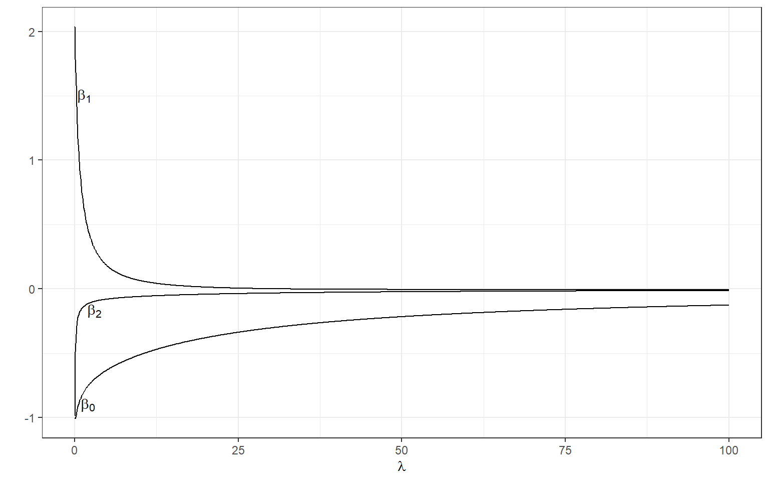
Standardized Variables
We haven’t considered a critical issue for the model estimation. This issue is not necessarily important if you have only one predictor; however, it is critical whenever you have more than one predictor. Different variables have different scales, and therefore the magnitude of the regression coefficients for different variables will depend on the variables’ scales. A regression coefficient for a predictor with a range from 0 to 100 will be very different from a regression coefficient for a predictor from 0 to 1. Therefore, if we work with the unstandardized variables, the ridge penalty will be amplified for the coefficients of those variables with a more extensive range of values.
Therefore, we must standardize variables before we use ridge regression. Let’s do the example in the previous section, but we now first standardize the variables in our model.
Y <-  as.matrix(readability_sub$target)
X <-  as.matrix(cbind(readability_sub$V220,readability_sub$V166))

# Standardize Y

  Y <- scale(Y)

  Y
[,1]
[1,] -1.34512103
[2,] 1.39315702
[3,] -0.92104526
[4,] -0.11446655
[5,] -1.01147297
[6,] -2.97759768
[7,] 0.14541127
[8,] 0.43376355
[9,] -0.37229209
[10,] -0.24350754
[11,] -0.11722056
[12,] 0.75591253
[13,] 0.27743280
[14,] 0.91902756
[15,] 0.89029923
[16,] 1.18783003
[17,] 0.18827737
[18,] 0.43482354
[19,] 0.38586691
[20,] 0.09092186
attr(,"scaled:center")
[1] -0.7633224
attr(,"scaled:scale")
[1] 0.9660852# Standardized X
X <- scale(X)
X [,1] [,2]
[1,] -1.54285661 1.44758852
[2,] 0.24727019 -0.47711825
[3,] -0.55323997 -0.97867834
[4,] -0.71812450 1.41817232
[5,] 0.28072891 -0.62244962
[6,] -1.23609737 0.11236158
[7,] 1.33304531 0.34607530
[8,] -2.06757849 -1.22697345
[9,] -0.04732188 0.05882229
[10,] -0.11743882 -1.24554362
[11,] 0.87248435 1.93772977
[12,] 0.42065052 0.13025831
[13,] -0.66763117 -0.40479141
[14,] 0.98226625 1.39073712
[15,] 0.65999286 0.25182543
[16,] 0.15056337 -0.28808443
[17,] -0.45313072 0.02862469
[18,] -0.44667480 0.25187100
[19,] 2.01553800 -2.00805114
[20,] 0.88755458 -0.12237606
attr(,"scaled:center")
[1] 0.1683671 0.1005784
attr(,"scaled:scale")
[1] 0.19927304 0.06196686When we standardize the variables, the mean of all variables becomes zero. So, the intercept estimate for any regression model with standardized variables is guaranteed to be zero. Note that our design matrix doesn’t have a column of ones because it is unnecessary (it would be a column of zeros if we had one).
First, check the regression model’s coefficients with standardized variables when there is no ridge penalty.
            [,1]
[1,]  0.42003881
[2,] -0.06335594
Now, let’s increase the ridge penalty to 0.5.
            [,1]
[1,]  0.40931629
[2,] -0.06215875
Below, we can manipulate the value of λ from 0 to 100 with increments of .1 as we did before and calculate the standardized regression coefficients.
Y <-  as.matrix(readability_sub$target)
X <-  as.matrix(cbind(readability_sub$V220,readability_sub$V166))

Y <- scale(Y)
X <- scale(X)

lambda <- seq(0,100,.1)

beta     <- data.frame(matrix(nrow=length(lambda),ncol=3))
beta[,1] <- lambda

for(i in 1:length(lambda)){
  beta[i,2:3] <- t(solve(t(X)%*%X + lambda[i]*diag(ncol(X)))%*%t(X)%*%Y)
}

ggplot(data = beta)+
  geom_line(aes(x=X1,y=X2))+
  geom_line(aes(x=X1,y=X3))+
  xlab(expression(lambda))+
  ylab('')+
  theme_bw()+
  geom_hline(yintercept=0,lty=2) +
  annotate(geom='text',x=3,y=.4,label=expression(beta[1]))+
  annotate(geom='text',x=2,y=-.075,label=expression(beta[2]))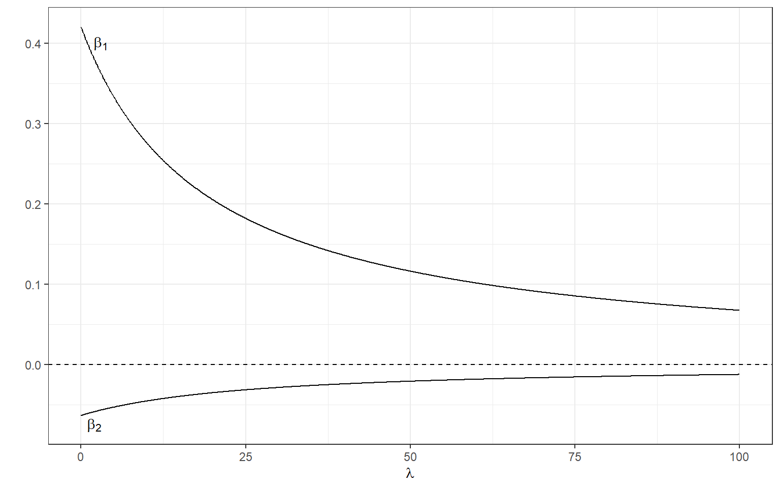
glmnet() function
Similar to the lm function, we can use the
glmnet() function from the glmnet package to
run a regression model with ridge penalty. There are many arguments for
the glmnet() function. For now, the arguments we need to
know are
x: an N x P input matrix, where N is the number of observations and P is the number of predictorsy: an N x 1 input matrix for the outcome variablealpha: a mixing constant for lasso and ridge penalty. When it is zero, the ridge regression is conductedlambda: penalty termintercept: set FALSE to avoid intercept for standardized variables
If you want to fit the linear regression without regularization, you
can specify alpha = 0 and lambda = 0.
#install.packages('glmnet')

require(glmnet)

Y <-  as.matrix(readability_sub$target)
X <-  as.matrix(cbind(readability_sub$V220,readability_sub$V166))
Y <- scale(Y)
X <- scale(X)

mod <- glmnet(x = X,
              y = Y,
              family = 'gaussian',
              alpha = 0,
              lambda = 0,
              intercept=FALSE)


coef(mod)
3 x 1 sparse Matrix of class "dgCMatrix"
s0
(Intercept) .
V1 0.42003881
V2 -0.06335594We can also increase the penalty term (λ).
#install.packages('glmnet')

require(glmnet)

Y <-  as.matrix(readability_sub$target)
X <-  as.matrix(cbind(readability_sub$V220,readability_sub$V166))
Y <- scale(Y)
X <- scale(X)

mod <- glmnet(x = X,
              y = Y,
              family = 'gaussian',
              alpha = 0,
              lambda = 0.5,
              intercept=FALSE)


coef(mod)
3 x 1 sparse Matrix of class "dgCMatrix"
s0
(Intercept) .
V1 0.27809880
V2 -0.04571182A careful eye should catch the fact that the coefficient estimates we
obtained from the glmnet() function for the two
standardized variables (Feature 220 and Feature 166) are different than
our matrix calculations above when the penalty term (λ) is 0.5. When we apply the matrix
solution above for the ridge regression, we obtained the estimates of
0.409 and -0.062 for the two predictors, respectively, at λ = 0.5. When we enter the same
value in glmnet(), we obtain the estimates of 0.278 and
-0.046. So, what is wrong? Where does this discrepancy come from?
There is nothing wrong. It appears that what lambda
argument in glmnet indicates is λN. In most statistics
textbooks, the penalty term for the ridge regression is specified as
λP∑i=1β2p.
On the other hand, if we examine Equation 1-3 in this paper
written by the developers of the glmnet package, we can see
that the penalty term applied is equivalent of
λNP∑i=1β2p.
Therefore, if we want identical results, we should use λ = 0.5/20.
N = 20

mod <- glmnet(x = X,
              y = Y,
              family = 'gaussian',
              alpha = 0,
              lambda = 0.5/N,
              intercept=FALSE)


coef(mod)
3 x 1 sparse Matrix of class "dgCMatrix"
s0
(Intercept) .
V1 0.40958102
V2 -0.06218857Note that these numbers are still slightly different. We can
attribute this difference to the numerical approximation
glmnet is using when optimizing the loss function.
glmnet doesn’t use the closed-form matrix solution for
ridge regression. This is a good thing because there is not always a
closed form solution for different types of regularization approaches
(e.g., lasso). Therefore, the computational approximation in
glmnet is very needed moving forward.
Tuning the Hyperparameter λ
In ridge regression, the λ parameter is called a hyperparameter. In the context of machine learning, the parameters in a model can be classified into two types: parameters and hyperparameters. The parameters are typically estimated from data and not set by users. In the context of ridge regression, regression coefficients, {β0,β1,...,βP}, are parameters to be estimated from data. On the other hand, the hyperparameters are not estimable, most of the time, because there are no first-order or second-order derivatives for these hyperparameters. Therefore, they must be set by the users. In the context of ridge regression, the penalty term, {λ}, is a hyperparameter.
The process of deciding what value to use for a hyperparameter is called tuning, and it is usually a trial-error process. The idea is simple. We try many different hyperparameter values and check how well the model performs based on specific criteria (e.g., MAE, MSE, RMSE) using k-fold cross-validation. Then, we pick the value of a hyperparameter that provides the best performance.
Using Ridge Regression to Predict Readability Scores
Please review the following notebook for applying Ridge Regresison to predict readability scores from all 768 features using the whole dataset.
Predicting Readability Scores using the Ridge Regression
Lasso Regression
Lasso regression is very similar to the Ridge regression. The only difference is that it applies a different penalty to the loss function. Assuming that there are P regression coefficients in the model, the penalty term for the ridge regression would be
λP∑i=1|βp|,
where λ is again the penalty constant and |βp| is the absolute value of the regression coefficient for the pth parameter. Lasso regression also penalizes the regression coefficients when they get larger but differently. When we fit a regression model with a lasso penalty, the loss function to minimize becomes
Loss=N∑i=1ϵ2(i)+λP∑i=1|βp|,
Loss=SSR+λP∑i=1|βp|.
Let’s consider the same example where we fit a simple linear regression model: the readability score is the outcome (Y) and Feature 229 is the predictor(X). Our regression model is
Y=β0+β1X+ϵ,
and let’s assume the set of coefficients are {β0,β1} = {-1.5,2}, so my model
is Y=−1.5+2X+ϵ.
Then, the value of the loss function when λ=0.2 would equal 18.467.
readability_sub <- read.csv('./data/readability_sub.csv',header=TRUE)

d <-  readability_sub[,c('V220','target')]

b0 = -1.5
b1 = 2

d$predicted <- b0 + b1*d$V220
d$error     <- d$target - d$predicted

d
V220 target predicted error
1 -0.13908258 -2.06282395 -1.7781652 -0.28465879
2 0.21764143 0.58258607 -1.0647171 1.64730321
3 0.05812133 -1.65313060 -1.3837573 -0.26937327
4 0.02526429 -0.87390681 -1.4494714 0.57556460
5 0.22430885 -1.74049148 -1.0513823 -0.68910918
6 -0.07795373 -3.63993555 -1.6559075 -1.98402809
7 0.43400714 -0.62284268 -0.6319857 0.00914304
8 -0.24364550 -0.34426981 -1.9872910 1.64302120
9 0.15893717 -1.12298826 -1.1821257 0.05913740
10 0.14496475 -0.99857142 -1.2100705 0.21149908
11 0.34222975 -0.87656742 -0.8155405 -0.06102693
12 0.25219145 -0.03304643 -0.9956171 0.96257066
13 0.03532625 -0.49529863 -1.4293475 0.93404886
14 0.36410633 0.12453660 -0.7717873 0.89632394
15 0.29988593 0.09678258 -0.9002281 0.99701073
16 0.19837037 0.38422270 -1.1032593 1.48748196
17 0.07807041 -0.58143038 -1.3438592 0.76242880
18 0.07935690 -0.34324576 -1.3412862 0.99804044
19 0.57000953 -0.39054205 -0.3599809 -0.03056111
20 0.34523284 -0.67548411 -0.8095343 0.13405021[1] 18.46657When λ is equal to 0, the loss function is again identical to SSR; therefore, it becomes a linear regression with no regularization. Below is a demonstration of what happens to the loss function and the regression coefficients for increasing levels of loss penalty (λ).
Model Estimation
Unfortunately, there is no closed-form solution for lasso regression
due to the absolute value terms in the loss function. The only way to
estimate the coefficients of the lasso regression is to optimize the
loss function using numerical techniques and obtain computational
approximations of the regression coefficients. Similar to ridge
regression, glmnet is an engine we can use to estimate the
coefficients of the lasso regression.
glmnet() function
We can fit the lasso regression by setting the alpha=
argument to 1 in glmnet() and specifying the penalty term
(λ).
Y <-  as.matrix(readability_sub$target)
X <-  as.matrix(cbind(readability_sub$V220,readability_sub$V166))
Y <- scale(Y)
X <- scale(X)

mod <- glmnet(x = X,
              y = Y,
              family = 'gaussian',
              alpha = 1,
              lambda = 0.2,
              intercept=FALSE)


coef(mod)
3 x 1 sparse Matrix of class "dgCMatrix"
s0
(Intercept) .
V1 0.2174345
V2 . Notice that there is a . symbol for the coefficient of
the second predictor. The . symbol indicates that it is
equal to zero. While the regression coefficients in the ridge regression
shrink to zero, they do not necessarily end up being exactly equal to
zero. In contrast, lasso regression may yield a value of zero for some
coefficients in the model. For this reason, lasso regression may be used
as a variable selection algorithm. The variables with coefficients equal
to zero may be discarded from future considerations as they are not
crucial for predicting the outcome.
Tuning λ
We implement a similar strategy for finding the optimal value of λ. We try many different values of λ and check how well the model performs based on specific criteria (e.g., MAE, MSE, RMSE) using k-fold cross-validation. Then, we pick the value of λ that provides the best performance.
Using Lasso Regression to Predict the Readability Scores
Please review the following notebook for applying Lasso Regresison to predict readability scores from all 768 features using the whole dataset.
Predicting Readability Scores using the Lasso Regression
Elastic Net
Elastic net combines the two types of penalty into one by mixing them with some weighted average. The penalty term for the elastic net could be written as
λ[(1−α)P∑i=1β2p+αP∑i=1|βp|)].
Note that this term reduces to
λP∑i=1β2p
when α is equal to 1 and to
λP∑i=1|βp|
when α is equal to 0.
When α is set to 1, this is equivalent to ridge regression. When α equals 0, this is the equivalent of lasso regression. When α takes any value between 0 and 1, this term becomes a weighted average of the ridge penalty and lasso penalty. In Elastic Net, two hyperparameters will be tuned, α and λ. We can consider all possible combinations of these two hyperparameters and try to find the optimal combination using 10-fold cross-validation.
Using Elastic Net to Predict the Readability Scores
Please review the following notebook for applying Elastic Net to predict readability scores from all 768 features using the whole dataset.
Predicting Readability Scores using the Elastic Net
Using the Prediction Model for a New Text
Please review the following notebook for predicting the readability of a given text with the existing model objects