An Overview of the Logistic Regression and Regularization

[Updated: Sun, Nov 27, 2022 - 14:05:58 ]

1. Overview of the Logistic Regression

Logistic regression is a type of model that can be used to predict a binary outcome variable. Linear and logistic regression are indeed members of the same family of models called generalized linear models. While linear regression can also technically be used to predict a binary outcome, the bounded nature of a binary outcome, [0,1], makes the linear regression solution suboptimal. Logistic regression is a more appropriate model that considers the bounded nature of the binary outcome when making predictions.

The binary outcomes can be coded in various ways in the data, such as 0 vs. 1, True vs. False, Yes vs. No, and Success vs. Failure. The rest of the notes assume that the outcome variable is coded as 0s and 1s. We are interested in predicting the probability that future observation will belong to the class of 1s. The notes in this section will first introduce a suboptimal solution to predict a binary outcome by fitting a linear probability model using linear regression and discuss the limitations of this approach. Then, the logistic regression model and its estimation will be demonstrated. Finally, we will discuss various metrics that can be used to evaluate the performance of a logistic regression model.

Throughout these notes, we will use the Recidivism dataset from the NIJ competition to discuss different aspects of logistic regression and demonstrations. This data and variables in this data were discussed in detail in Lecture 1 and Lecture 2a – Section 6. The outcome of interest to predict in this dataset is whether or not an individual will be recidivated in the second year after initial release. To make demonstrations easier, I randomly sample 20 observations from this data. Eight observations in this data have a value of 1 for the outcome (recidivated), and 12 observations have a value of 0 (not recidivated).

# Import the randomly sample 20 observations from the recidivism dataset

recidivism_sub <- read.csv('./data/recidivism_sub.csv',header=TRUE)

# Outcome variable

table(recidivism_sub$Recidivism_Arrest_Year2)

 0  1 
12  8 

1.1. Linear Probability Model

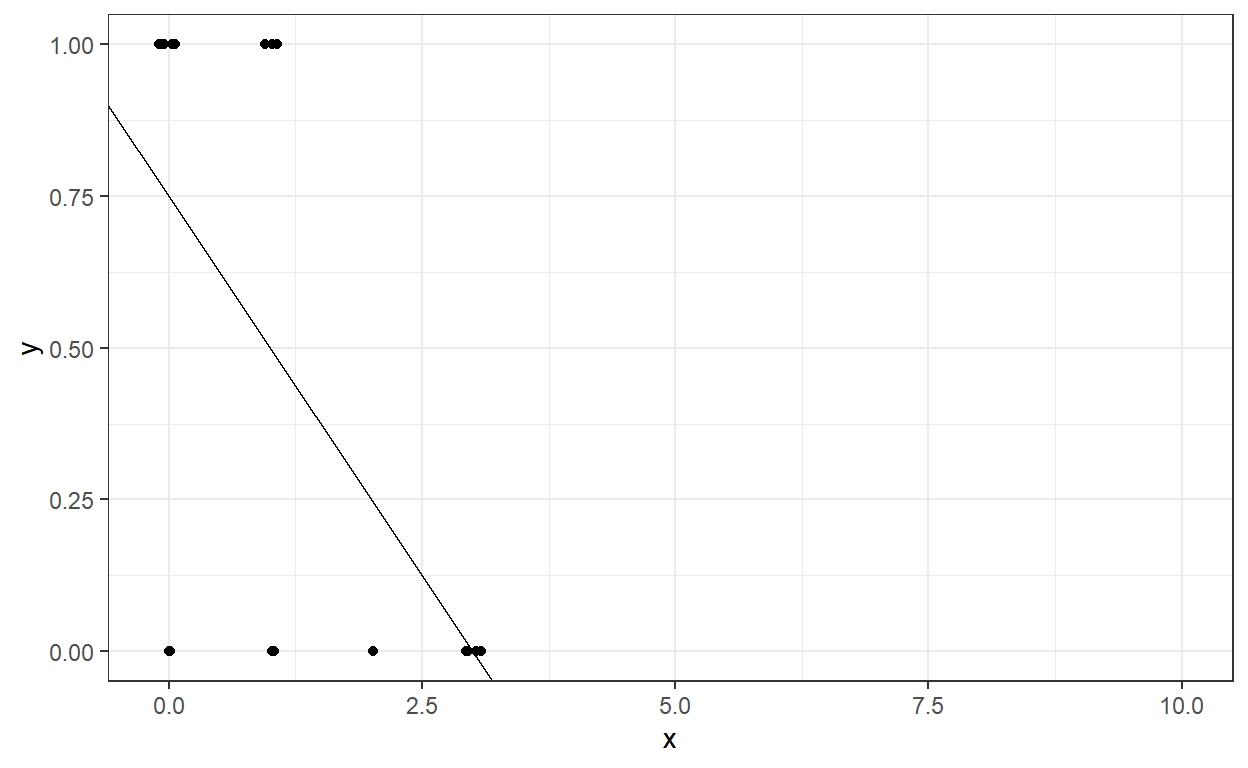
A linear probability model fits a typical regression model to a binary outcome. When the outcome is binary, the predictions from a linear regression model can be considered as the probability of the outcome being equal to 1,

ˆY=P(Y=1).

Suppose we want to predict the recidivism in the second year (Recidivism_Arrest_Year2) by using the number of dependents they have. Then, we could fit this using the lm function.

ˆY=P(Y=1)=β0+β1X+ϵ

mod <- lm(Recidivism_Arrest_Year2 ~ 1 + Dependents,
          data = recidivism_sub)
summary(mod)

Call:
lm(formula = Recidivism_Arrest_Year2 ~ 1 + Dependents, data = recidivism_sub)

Residuals:
    Min      1Q  Median      3Q     Max 
-0.7500 -0.0625  0.0000  0.2500  0.5000 

Coefficients:
            Estimate Std. Error t value  Pr(>|t|)    
(Intercept)  0.75000    0.12949   5.792 0.0000173 ***
Dependents  -0.25000    0.06825  -3.663   0.00178 ** 
---
Signif. codes:  0 '***' 0.001 '**' 0.01 '*' 0.05 '.' 0.1 ' ' 1

Residual standard error: 0.3909 on 18 degrees of freedom
Multiple R-squared:  0.4271,    Adjusted R-squared:  0.3953 
F-statistic: 13.42 on 1 and 18 DF,  p-value: 0.001779

The intercept is 0.75 and the slope for the predictor, Dependents, is -.25. We can interpret the intercept and slope as the following for this example. Note that the predicted values from this model can now be interpreted as probability predictions because the outcome is binary.

• Intercept (0.75): When the number of dependents is equal to 0, the probability of being recidivated in Year 2 is 0.75.

• Slope (-0.25): For every additional dependent (one unit increase in X) the individual has, the probability of being recidivated in Year 2 is reduced by .25.

The intercept and slope still represent the best-fitting line to our data, and this fitted line can be shown here.

Suppose we want to calculate the model’s predicted probability of being recidivated in Year 2 for a different number of dependents a parolee has. Let’s assume that the number of dependents can be from 0 to 10. What would be the predicted probability of being recidivated in Year 2 for a parolee with eight dependents?

X <- data.frame(Dependents = 0:10)
predict(mod,newdata = X)

                        1                         2 
 0.7500000000000000000000  0.4999999999999999444888 
                        3                         4 
 0.2499999999999998889777 -0.0000000000000002220446 
                        5                         6 
-0.2500000000000002220446 -0.5000000000000002220446 
                        7                         8 
-0.7500000000000004440892 -1.0000000000000004440892 
                        9                        10 
-1.2500000000000004440892 -1.5000000000000004440892 
                       11 
-1.7500000000000004440892 

It is not reasonable for a probability prediction to be negative. One of the major issues with using linear regression to predict a binary outcome using a linear-probability model is that the model predictions can go outside of the boundary [0,1] and yield unreasonable predictions. So, a linear regression model may not be the best tool to predict a binary outcome. We should use a model that respects the boundaries of the outcome variable.

1.2. Description of Logistic Regression Model

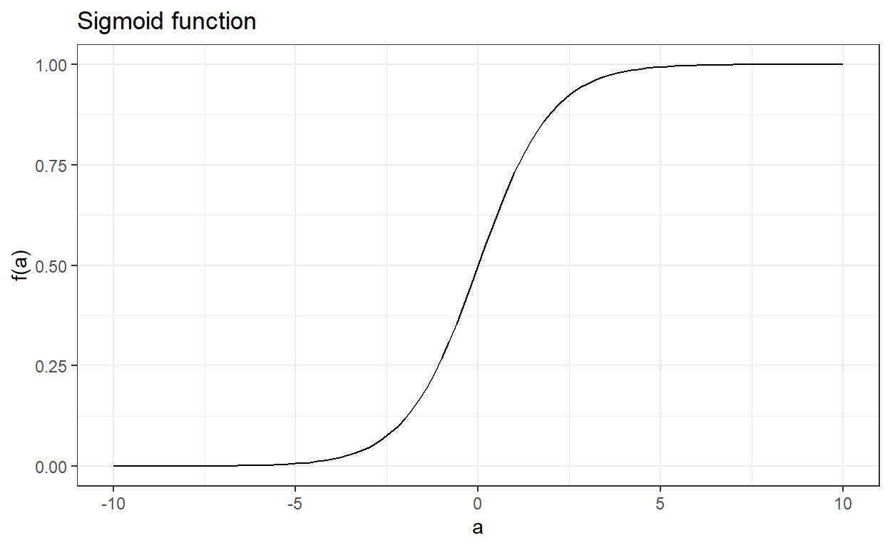
To overcome the limitations of the linear probability model, we bundle our prediction model in a sigmoid function. Suppose there is a real-valued function of a such that

f(a)=ea1+ea.

The output of this function is always between 0 and 1 regardless of the value of a. The sigmoid function is an appropriate choice for the logistic regression because it assures that the output is always bounded between 0 and 1.

Note that this function can also be written as the following, and they are mathematically equivalent.

f(a)=11+e−a.

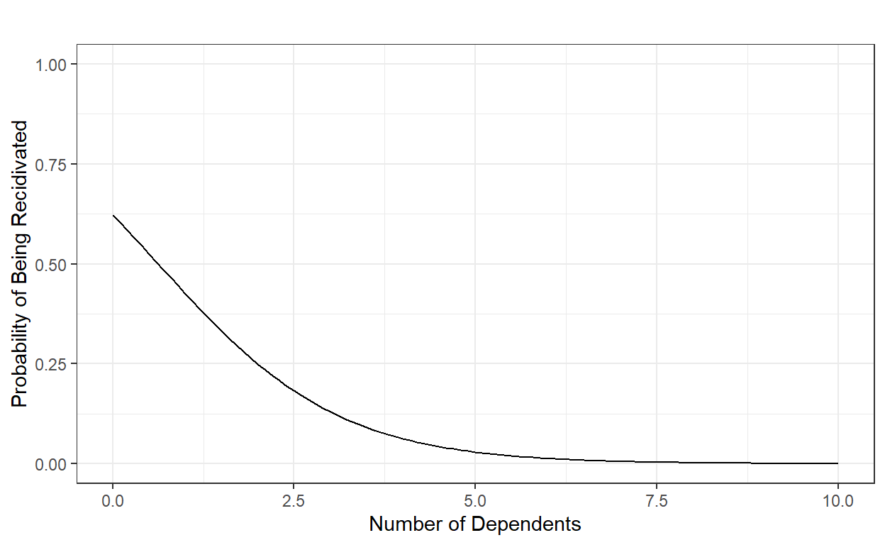
If we revisit the previous example, we can specify a logistic regression model to predict the probability of being recidivated in Year 2 as the following by using the number of dependents a parolee has as the predictor,

P(Y=1)=11+e−(β0+β1X).

When values of a predictor variable is entered into the equation, the model output can be directly interpreted as the probability of the binary outcome being equal to 1 (or whatever category and meaning a value of 1 represents). Then, we assume that the actual outcome follows a binomial distribution with the predicted probability.

P(Y=1)=p

Y∼Binomial(p)

Suppose the coefficient estimates of this model are β0=1.33 and β1=-1.62. Then, for instance, we can compute the probability of being recidivated for a parolee with 8 dependents as the following:

P(Y=1)=11+e−(1.33−1.62×8)=0.0000088951098.

b0 = 1.33
b1 = -1.62
x = 0:10
y = 1/(1+exp(-(b0+b1*x)))
data.frame(number.of.dependents = x, probability=y)

   number.of.dependents     probability
1                     0 0.7908406347869
2                     1 0.4280038670685
3                     2 0.1289808521462
4                     3 0.0284705876901
5                     4 0.0057659655589
6                     5 0.0011463789579
7                     6 0.0002270757033
8                     7 0.0000449461727
9                     8 0.0000088951098
10                    9 0.0000017603432
11                   10 0.0000003483701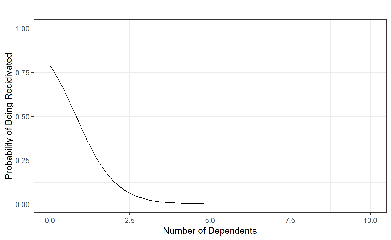

In its original form, it is difficult to interpret the logistic regression parameters because a one unit increase in the predictor is no longer linearly related to the probability of the outcome being equal to 1 due to the nonlinear nature of the sigmoid function.

The most common presentation of logistic regression is obtained after a bit of algebraic manipulation to rewrite the model equation. The logistic regression model above can also be specified as the following without any loss of meaning as they are mathematically equivalent.

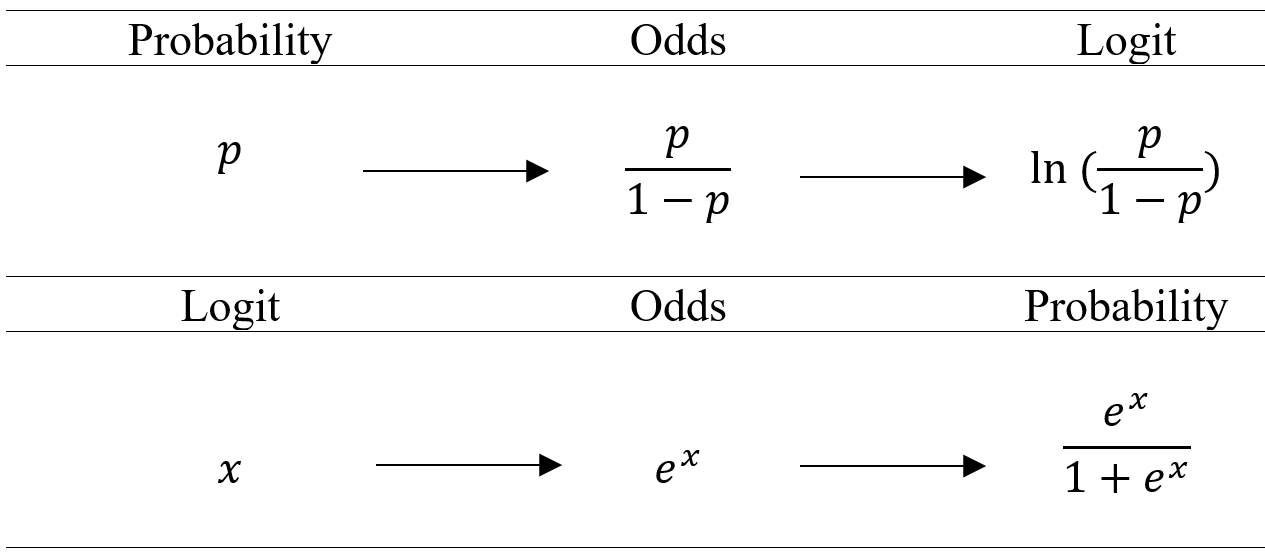
ln[P(Y=1)1−P(Y=1)]=β0+β1X.

The term on the left side of the equation is known as the logit. It is essentially the natural logarithm of odds. So, when the outcome is a binary variable, the logit transformation of the probability that the outcome is equal to 1 can be represented as a linear equation. It provides a more straightforward interpretation. For instance, we can now say that when the number of dependents is equal to zero, the predicted logit is equal to 1.33 (intercept), and for every additional dependent, the logit decreases by 1.62 (slope).

It is common to transform the logit to odds when interpreting the parameters. For instance, we can say that when the number of dependents is equal to zero, the odds of being recidivated is 3.78 (e1.33), and for every additional dependent the odds of being recidivated is reduced by about 80% (1−e−1.62).

The right side of the equation can be expanded by adding more predictors, adding polynomial terms of the predictors, or adding interactions among predictors. A model with only the main effects of P predictors can be written as

ln[P(Y=1)1−P(Y=1)]=β0+P∑p=1βpXp, and the coefficients can be interpreted as

• β0: the predicted logit when the values for all the predictor variables in the model are equal to zero. eβ0, the predicted odds of the outcome being equal to 1 when the values for all the predictor variables in the model are equal to zero.

• βp: the change in the predicted logit for one unit increases in Xp when the values for all other predictors in the model are held constant. For every one unit in increase in Xp, the odds of the outcome being equal to 1 is multiplied by eβp when the values for all other predictors in the model are held constant. In other words, eβp is odds ratio, the ratio of odds at βp=a+1 to the odds at βp=a.

It is essential that you get familiar with the three concepts (probability, odds, logit) and how these three are related to each other for interpreting the logistic regression parameters.

---

NOTE

The sigmoid function is not the only tool to be used for modeling a binary outcome. One can also use the cumulative standard normal distribution function, ϕ(a), and the output of ϕ(a) is also bounded between 0 and 1. When ϕ is used to transform the prediction model, this is known as probit regression and serves the same purpose as the logistic regression, which is to predict the probability of a binary outcome being equal to 1. However, it is always easier and more pleasant to work with logarithmic functions, which have better computational properties. Therefore, logistic regression is more commonly used than probit regression.

---

1.3. Model Estimation

1.3.1. The concept of likelihood

It is essential to understand the likelihood concept for estimating the coefficients of a logistic regression model. We will consider a simple example of flipping coins for this.

Suppose you flip the same coin 20 times and observe the following outcome. We don’t know whether this is a fair coin in which the probability of observing a head or tail is equal to 0.5.

Y=(H,H,H,T,H,H,H,T,H,T)

Suppose we define p as the probability of observing a head when we flip this coin. By definition, the probability of observing a tail is 1−p.

P(Y=H)=p

P(Y=T)=1−p

Then, we can calculate the likelihood of our observations of heads and tails as a function of p.

L(Y|p)=p×p×p×(1−p)×p×p×p×(1−p)×p×(1−p)

L(Y|p)=p7×(1−p)3 For instance, if we say that this is a fair coin and, therefore, p is equal to 0.5, then the likelihood of observing seven heads and three tails would be equal to

L(Y|p=0.5)=0.57×(1−0.5)3=0.0009765625 On the other hand, another person can say this is probably not a fair coin, and the p should be something higher than 0.5. How about 0.65?

L(Y|p=0.65)=0.657×(1−0.65)3=0.00210183 Based on our observation, we can say that an estimate of p being equal to 0.65 is more likely than an estimate of p being equal to 0.5. Our observation of 7 heads and 3 tails is more likely if we estimate p as 0.65 rather than 0.5.

1.3.2. Maximum likelihood estimation (MLE)

Then, what would be the best estimate of p given our observed data (seven heads and three tails)? We can try every possible value of p between 0 and 1 and calculate the likelihood of our data (Y). Then, we can pick the value that makes our data most likely (largest likelihood) to observe as our best estimate. Given the data we observed (7 heads and three tails), it is called the maximum likelihood estimate of p.

p <- seq(0,1,.001)

L <- p^7*(1-p)^3

ggplot()+
  geom_line(aes(x=p,y=L)) + 
  theme_bw() + 
  xlab('Probability of Observing a Head (p)')+
  ylab('Likelihood of Observing 7 Heads and 3 Tails')+
  geom_vline(xintercept=p[which.max(L)],lty=2)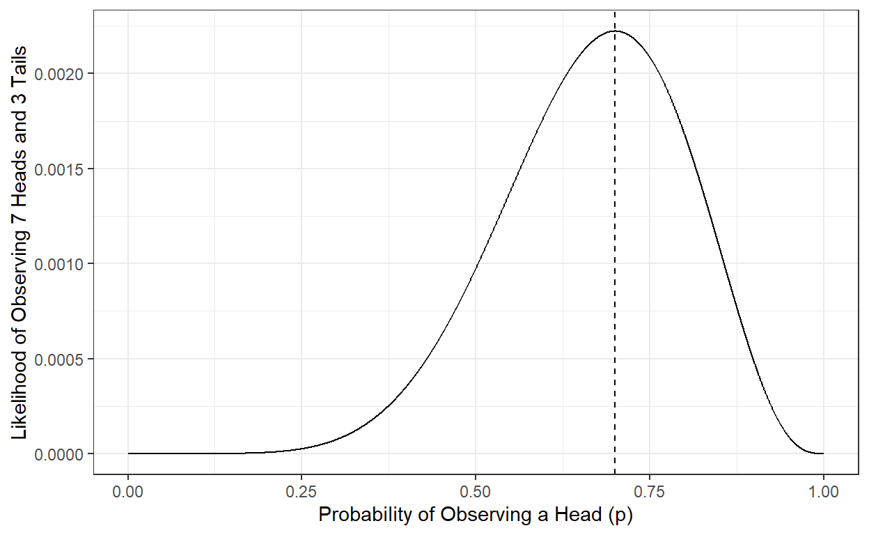

We can show that the p value that makes the likelihood largest is 0.7, and the likelihood of observing seven heads and three tails is 0.002223566 when p is equal to 0.7. Therefore, the maximum likelihood estimate of the probability of observing a head for this particular coin is 0.7, given the ten observations we have made.

L[which.max(L)]

[1] 0.002223566

p[which.max(L)]

[1] 0.7

Note that our estimate can change and be updated if we continue collecting more data by flipping the same coin and recording our observations.

1.3.3. The concept of the log-likelihood

The computation of likelihood requires the multiplication of so many p values, and when you multiply values between 0 and 1, the result gets smaller and smaller. It creates problems when you multiply so many of these small p values due to the maximum precision any computer can handle. For instance, you can see the minimum number that can be represented in R in your local machine.

.Machine$double.xmin

[1] 2.225074e-308

When you have hundreds of thousands of observations, it is probably not a good idea to work directly with likelihood. Instead, we work with the log of likelihood (log-likelihood). The log-likelihood has two main advantages:

• We are less concerned about the precision of small numbers our computer can handle.

• Log-likelihood has better mathematical properties for optimization problems (the log of the product of two numbers equals the sum of the log of the two numbers).

• The point that maximizes likelihood is the same number that maximizes the log-likelihood, so our end results (MLE estimate) do not care if we use log-likelihood instead of likelihood.

ln(L(Y|p))=ln(lop7×(1−p)3) ln(L(Y|p))=ln(p7)+ln((1−p)3) ln(L(Y|p))=7×ln(p)+3×ln(1−p)

p <- seq(0,1,.001)

logL <- log(p)*7 + log(1-p)*3

ggplot()+
  geom_line(aes(x=p,y=logL)) + 
  theme_bw() + 
  xlab('Probability of Observing a Head (p)')+
  ylab('Loglikelihood of Observing 7 Heads and 3 Tails')+
  geom_vline(xintercept=p[which.max(logL)],lty=2)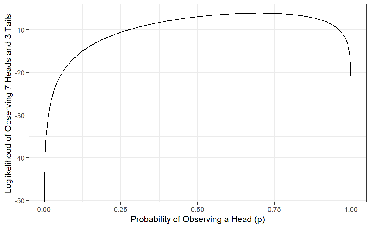

logL[which.max(logL)]

[1] -6.108643

p[which.max(logL)]

[1] 0.7

1.3.4. MLE for Logistic Regression coefficients

Now, we can apply these concepts to estimate the logistic regression coefficients. Let’s revisit our previous example in which we predict the probability of being recidivated in Year 2, given the number of dependents a parolee has. Our model can be written as the following.

ln[Pi(Y=1)1−Pi(Y=1)]=β0+β1Xi.

Note that X and P have a subscript i to indicate that each individual may have a different X value, and therefore each individual will have a different probability. Our observed outcome is a set of 0s and 1s. Remember that eight individuals were recidivated (Y=1), and 12 were not recidivated (Y=0).

recidivism_sub$Recidivism_Arrest_Year2

 [1] 1 1 0 0 1 1 1 1 0 0 0 0 1 0 0 1 0 0 0 0

Given a set of coefficients, {β0,β1}, we can calculate the logit for every observation using the model equation and then transform this logit to a probability, Pi(Y=1). Finally, we can calculate the log of the probability for each observation and sum them across observations to obtain the log-likelihood of observing this set of observations (12 zeros and eight ones). Suppose that we have two guesstimates for {β0,β1}, which are 0.5 and -0.8, respectively. These coefficients imply the following predicted model.

If these two coefficients were our estimates, how likely would we observe the outcome in our data, given the number of dependents? The below R code first finds the predicted logit for every observation, assuming that β0 = 0.5 and β1 = -0.8.

b0 = 0.5
b1 = -0.8

x = recidivism_sub$Dependents

y = recidivism_sub$Recidivism_Arrest_Year2

pred_logit <- b0 + b1*x

pred_prob1 <- exp(pred_logit)/(1+exp(pred_logit))

pred_prob0 <- 1 - pred_prob1 

data.frame(Dependents      = x, 
           Recidivated     = y, 
           Prob1 = pred_prob1,
           Prob0 = pred_prob0)

   Dependents Recidivated     Prob1     Prob0
1           0           1 0.6224593 0.3775407
2           1           1 0.4255575 0.5744425
3           2           0 0.2497399 0.7502601
4           1           0 0.4255575 0.5744425
5           1           1 0.4255575 0.5744425
6           0           1 0.6224593 0.3775407
7           0           1 0.6224593 0.3775407
8           1           1 0.4255575 0.5744425
9           3           0 0.1301085 0.8698915
10          0           0 0.6224593 0.3775407
11          1           0 0.4255575 0.5744425
12          0           0 0.6224593 0.3775407
13          0           1 0.6224593 0.3775407
14          3           0 0.1301085 0.8698915
15          3           0 0.1301085 0.8698915
16          0           1 0.6224593 0.3775407
17          3           0 0.1301085 0.8698915
18          3           0 0.1301085 0.8698915
19          3           0 0.1301085 0.8698915
20          3           0 0.1301085 0.8698915

logL <-  y*log(pred_prob1) + (1-y)*log(pred_prob0)
sum(logL)

[1] -9.253358

We can summarize this by saying that if our model coefficients were β0 = 0.5 and β1 = -0.8, then the log of the likelihood of observing the outcome in our data would be -9.25.

Y=(1,0,1,0,0,0,0,1,1,0,0,1,0,0,0,1,0,0,0,0)

logL(Y|β0=0.5,β1=−0.8)=−9.25

The critical question is whether or not there is another pair of values we can assign to β0 and β1 that would provide a higher likelihood of data. If there are, then they would be better estimates for our model. If we can find such a pair with the maximum log-likelihood of data, then they would be our maximum likelihood estimates for the given model.

We can approach this problem crudely to gain some intuition about Maximum Likelihood Estimation. Suppose that a reasonable range of values for β0 is from -3 to 3, and for β1 is from -3 to 3. Let’s think about every possible combinations of values for β0 and β1 within these ranges with increments of .01. Then, let’s calculate the log-likelihood of data for every possible combination and plot these in a 3D plot as a function of β0 and β1.

grid    <- expand.grid(b0=seq(-3,3,.01),b1=seq(-3,3,.01))           

grid$logL <- NA

for(i in 1○:nrow(grid)){
  
  x = recidivism_sub$Dependents
  y = recidivism_sub$Recidivism_Arrest_Year2

  pred_logit    <- grid[i,]$b0 + grid[i,]$b1*x
  pred_prob1    <- exp(pred_logit)/(1+exp(pred_logit))
  pred_prob0    <- 1 - pred_prob1 
  logL          <- y*log(pred_prob1) + (1-y)*log(pred_prob0)
  grid[i,]$logL <- sum(logL)
  
  print(i)
}

  
require(plotly)

plot_ly(grid, x = ~b0, y = ~b1, z = ~logL, 
        marker = list(color = ~logL,
                      showscale = FALSE,
                      cmin=min(grid$logL),
                      cmax=max(grid$logL),cauto=F),
        width=600,height=600) %>% 
  add_markers()

What is the maximum point of this surface? Our simple search indicates that it is -8.30, and the set of β0 and β1 coefficients that make the observed data most likely is 1.33 and -1.62.

grid[which.max(grid$logL),]

        b0    b1      logL
83372 1.33 -1.62 -8.306004

Therefore, given our dataset with 20 observations, our maximum likelihood estimates for the coefficients of the logistic regression model above are 1.33 and -1.62.

ln[Pi(Y=1)1−Pi(Y=1)]=1.33−1.62×Xi.

1.3.5. Logistic Loss function

Below is a compact way of writing likelihood and log-likelihood in mathematical notation. For simplification purposes, we write Pi to represent Pi(Y=1).

L(Y|β)=N∏i=1Pyii×(1−Pi)1−yi

logL(Y|β)=N∑i=1Yi×ln(Pi)+(1−Yi)×ln(1−Pi)

The final equation above, logL(Y|β), is known as the logistic loss function.

By finding the set of coefficients in a model, β=(β0,β1,...,βP), that maximizes this quantity, we obtain the maximum likelihood estimates of the coefficients for the logistic regression model.

Unfortunately, the naive crude search we applied above would be inefficient when you have a complex model with many predictors. Another unfortunate thing is that there is no closed-form solution (as we had for the linear regression) for the logistic regression. Therefore, the only way to estimate the logistic regression coefficients is to use numerical approximations and computational algorithms to maximize the logistic loss function. Luckily, we have tools available to accomplish this task.

---

NOTE

Why do we not use least square estimation and minimize the sum of squared residuals when estimating the coefficients of the logistic regression model? We can certainly use the sum of squared residuals as our loss function and minimize it to estimate the coefficients for the logistic regression, just like we did for the linear regression. The complication is that the sum of the squared residuals function yields a non-convex surface when the outcome is binary as opposed to a convex surface obtained from the logistic loss function. Non-convex optimization problems are more challenging than convex optimization problems, and they are more vulnerable to finding sub-optimal solutions (local minima/maxima). Therefore, the logistic loss function and maximizing it is preferred when estimating the coefficients of a logistic regression model.

---

1.3.6. The glm function

The glm() function as a part of the base stats package can be used to estimate the logistic regression coefficients. The use of the glm() function is very similar to the lm() function. The only difference is that we specify the family='binomial' argument to fit the logistic regression by maximizing the logistic loss function.

mod <- glm(Recidivism_Arrest_Year2 ~ 1 + Dependents,
           data   = recidivism_sub,
           family = 'binomial')

summary(mod)

Call:
glm(formula = Recidivism_Arrest_Year2 ~ 1 + Dependents, family = "binomial", 
    data = recidivism_sub)

Deviance Residuals: 
    Min       1Q   Median       3Q      Max  
-1.7670  -0.3125  -0.2412   0.6864   1.3031  

Coefficients:
            Estimate Std. Error z value Pr(>|z|)  
(Intercept)   1.3255     0.8204   1.616   0.1061  
Dependents   -1.6161     0.7269  -2.223   0.0262 *
---
Signif. codes:  0 '***' 0.001 '**' 0.01 '*' 0.05 '.' 0.1 ' ' 1

(Dispersion parameter for binomial family taken to be 1)

    Null deviance: 26.920  on 19  degrees of freedom
Residual deviance: 16.612  on 18  degrees of freedom
AIC: 20.612

Number of Fisher Scoring iterations: 5

In the Coefficients table, the numbers under the Estimate column are the estimated coefficients for the logistic regression model. The quantity labeled as the Residual Deviance in the output is twice the maximized log-likelihood,

Deviance=−2×logL(Y|β).

Notice that the coefficient estimates from the glm() function are very close to our crude estimates from a brute-force search in an earlier section (1.33 and -1.62). From our simple search, we found the maximum log-likelihood as -8.3. So, if we multiply that number by -2, that equals 16.6, which is the number reported in this output as Residual Deviance.

1.3.7. The glmnet function

You can also use the glmnet() function from the glmnet package to fit the logistic regression. The advantage of the glmnet package is that it allows regularization while fitting the logistic regression. You can set the alpha=0 and lambda=0 arguments to obtain the coefficient estimates without penalty.

require(glmnet)

mod <- glmnet(x         = cbind(0,recidivism_sub$Dependents),
              y         = factor(recidivism_sub$Recidivism_Arrest_Year2),
              family    = 'binomial',
              alpha     = 0,
              lambda    = 0,
              intercept = TRUE)

coef(mod)

3 x 1 sparse Matrix of class "dgCMatrix"
                   s0
(Intercept)  1.325172
V1           .       
V2          -1.615664

The x argument is the input matrix for predictors, and the y' argument is a vector of binary response outcome. Theglmnetrequires they’ argument to be a factor with two levels.

Note that I defined the x argument above as cbind(0,recidivism_sub$Dependents) because glmnet requires the x to be a matrix with at least two columns. So, I added a column of zeros to trick the function and force it to run. That column of zeros has zero impact on the estimation.

1.4. Evaluating the Predictive Performance for Logistic Regression Models

When the outcome is a binary variable, classification models, such as logistic regression), typically yield a probability estimate for a class membership (or a continuous-valued prediction between 0 and 1).

For instance, we can obtain the model predictive probabilities of being recidivated in Year 2 after fitting a simple logistic regression as the number of dependents is the predictor.

mod <- glm(Recidivism_Arrest_Year2 ~ 1 + Dependents,
           data   = recidivism_sub,
           family = 'binomial')

recidivism_sub$pred_prob <- predict(mod,type='response')

recidivism_sub[,c('ID','Dependents','Recidivism_Arrest_Year2','pred_prob')]

      ID Dependents Recidivism_Arrest_Year2  pred_prob
1  21953          0                       1 0.79010012
2   8255          1                       1 0.42785504
3   9110          2                       0 0.12934698
4  20795          1                       0 0.42785504
5   5569          1                       1 0.42785504
6  14124          0                       1 0.79010012
7  24979          0                       1 0.79010012
8   4827          1                       1 0.42785504
9  26586          3                       0 0.02866814
10 17777          0                       0 0.79010012
11 22269          1                       0 0.42785504
12 25016          0                       0 0.79010012
13 24138          0                       1 0.79010012
14 12261          3                       0 0.02866814
15 15417          3                       0 0.02866814
16 14695          0                       1 0.79010012
17  4371          3                       0 0.02866814
18 13529          3                       0 0.02866814
19 25046          3                       0 0.02866814
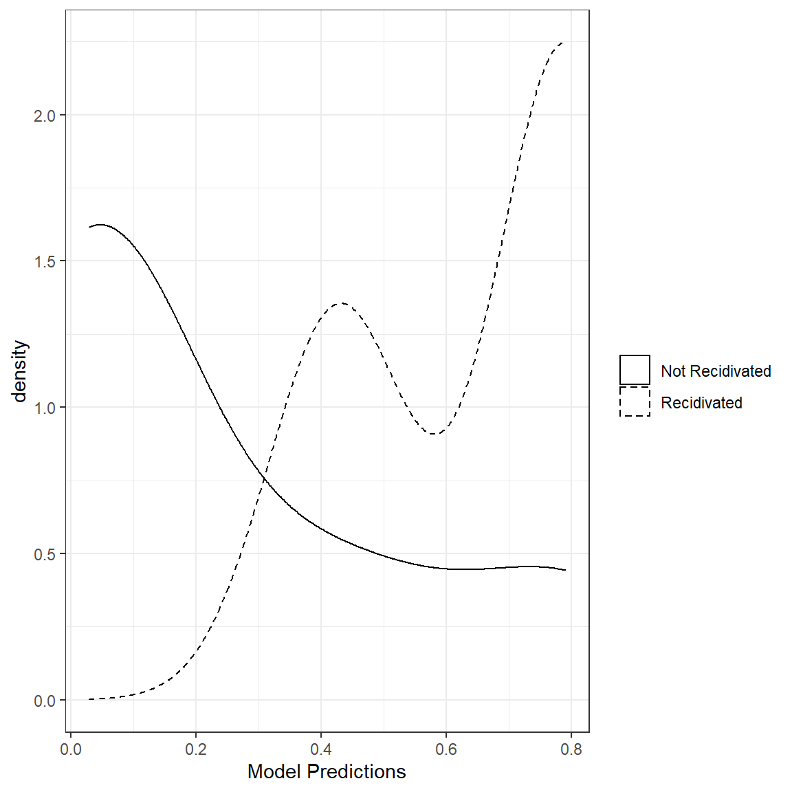
20  5340          3                       0 0.02866814

In an ideal situation where a model does a perfect job of predicting a binary outcome, we expect all those observations in Group 0 (Not Recidivated) to have a predicted probability of 0 and all those observations in Group 1 (Recidivated) to have a predicted probability of 1. So, predicted values close to 0 for observations in Group 0 and those close to 1 for Group 1 are desirable.

One way to look at the quality of predictions for a binary outcome is to examine the distribution of predictions for both categories of the outcome variable. For this small demo set with 20 observations, we can see that these distributions are not separated very well. This plot implies that our model predictions don’t properly separate the two classes in the outcome variable. The more separation between the distribution of two classes, the better the model performance is.

What would such a plot look like for a model with perfect classification?

This visualization is a very intuitive initial look at the model performance. Later, we will see numerical summaries of the separation between these two distributions.

1.4.1. Accuracy of Class Probabilities

We can calculate MAE and RMSE to measure the accuracy of predicted probabilities when the outcome is binary, and they have the same definition as in the continuous case.

outs  <- recidivism_sub$Recidivism_Arrest_Year2
preds <- recidivism_sub$pred_prob

# Mean absolute error

mean(abs(outs - preds))

[1] 0.2765934

# Root mean squared error

sqrt(mean((outs - preds)^2))

[1] 0.376793

1.4.2. Accuracy of Class Predictions

Confusion Matrix and Related Metrics

In most situations, the accuracy of class probabilities is not very useful because one has to decide and place these observations in a group based on these probabilities for practical reasons. For instance, suppose you are predicting whether or not an individual will be recidivated so you can take action based on this decision. Then, it would be best if you transformed this continuous probability (or probability-like score) predicted by a model into a binary prediction. Therefore, one has to determine an arbitrary cut-off value. Once a cut-off value is determined, then we can generate class predictions.

Consider that we use a cut-off value of 0.5. So, if an observation has a predicted class probability less than 0.5, we predict that this person is in Group 0 (Not Recidivated). Likewise, if an observation has a predicted class probability higher than 0.5, we predict that this person is in Group 1.

In the code below, I convert the class probabilities to class predictions using a cut-off value of 0.5.

recidivism_sub$pred_class <- ifelse(recidivism_sub$pred_prob>.5,1,0)

recidivism_sub[,c('ID','Dependents','Recidivism_Arrest_Year2','pred_prob','pred_class')]

      ID Dependents Recidivism_Arrest_Year2  pred_prob pred_class
1  21953          0                       1 0.79010012          1
2   8255          1                       1 0.42785504          0
3   9110          2                       0 0.12934698          0
4  20795          1                       0 0.42785504          0
5   5569          1                       1 0.42785504          0
6  14124          0                       1 0.79010012          1
7  24979          0                       1 0.79010012          1
8   4827          1                       1 0.42785504          0
9  26586          3                       0 0.02866814          0
10 17777          0                       0 0.79010012          1
11 22269          1                       0 0.42785504          0
12 25016          0                       0 0.79010012          1
13 24138          0                       1 0.79010012          1
14 12261          3                       0 0.02866814          0
15 15417          3                       0 0.02866814          0
16 14695          0                       1 0.79010012          1
17  4371          3                       0 0.02866814          0
18 13529          3                       0 0.02866814          0
19 25046          3                       0 0.02866814          0
20  5340          3                       0 0.02866814          0

We can summarize the relationship between the binary outcome and binary prediction in a 2 x 2 table. This table is commonly referred to as confusion matrix.

tab <- table(recidivism_sub$pred_class,
             recidivism_sub$Recidivism_Arrest_Year2,
             dnn = c('Predicted','Observed'))
tab

         Observed
Predicted  0  1
        0 10  3
        1  2  5

The table indicates that there are 12 observations with an outcome value of 0. The model accurately predicts the class membership as 0 for ten observation while inaccurately predicts class membership as 1 for two observations. The table also indicates that there are eight observations with an outcome value of 1. The model accurately predicts the class membership as 1 for 5 observations while inaccurately predicts class membership as 0 for three observations.

Based on the elements of this table, we can define four key concepts:

• True Positives(TP): True positives are the observations where both the outcome and prediction are equal to 1.

• True Negative(TN): True negatives are the observations where both the outcome and prediction are equal to 0.

• False Positives(FP): False positives are the observations where the outcome is 0 but the prediction is 1.

• False Negatives(FN): False negatives are the observations where the outcome is 1 but the prediction is 0.

tn <- tab[1,1]
tp <- tab[2,2]
fp <- tab[2,1]
fn <- tab[1,2]

Several metrics can be defined based on these four variables. We define a few important metrics below.

• accuracy: Overall accuracy simply represent the proportion of correct predictions.

ACC=TP+TNTP+TN+FP+FN

acc <- (tp + tn)/(tp+tn+fp+fn)

acc

[1] 0.75

• True Positive Rate (Sensitivity): True positive rate (a.k.a. sensitivity) is the proportion of correct predictions for those observations the outcome is 1 (event is observed).

TPR=TPTP+FN

tpr <- (tp)/(tp+fn)

tpr

[1] 0.625

• True Negative Rate (Specificity): True negative rate (a.k.a. specificity) is the proportion of correct predictions for those observations the outcome is 0 (event is not observed).

TNR=TNTN+FP

tnr <- (tn)/(tn+fp)

tnr

[1] 0.8333333

• Positive predicted value (Precision): Positive predicted value (a.k.a. precision) is the proportion of correct decisions when the model predicts that the outcome is 1.

PPV=TPTP+FP

ppv <- (tp)/(tp+fp)

ppv

[1] 0.7142857

• F1 score: F1 score is a metric that combines both PPV and TPR.

F1=2∗PPV∗TPRPPV+TPR

f1 <- (2*ppv*tpr)/(ppv+tpr)

f1

[1] 0.6666667

Area Under the Receiver Operating Curve (AUC or AUROC)

The confusion matrix and related metrics all depend on the arbitrary cut-off value one picks when transforming continuous predicted probabilities to binary predicted classes. We can change the cut-off value to optimize certain metrics, and there is always a trade-off between these metrics for different cut-off values. For instance, let’s pick different cut-off values and calculate these metrics for each one.

# Write a generic function to return the metric for a given vector of observed 
# outcome, predicted probability and cut-off value

cmat <- function(x,y,cut){
  # x, a vector of predicted probabilities
  # y, a vector of observed outcomes
  # cut, user-defined cut-off value
 
  x_ <- ifelse(x>cut,1,0)
    
  tn <- sum(x_==0 & y==0)
  tp <- sum(x_==1 & y==1)
  fp <- sum(x_==1 & y==0)
  fn <- sum(x_==0 & y==1)
  
  acc <- (tp + tn)/(tp+tn+fp+fn)
  tpr <- (tp)/(tp+fn)
  tnr <- (tn)/(tn+fp)
  ppv <- (tp)/(tp+fp)
  f1 <- (2*ppv*tpr)/(ppv+tpr)

  return(list(acc=acc,tpr=tpr,tnr=tnr,ppv=ppv,f1=f1))
}

# Try it out

  #cmat(x=recidivism_sub$pred_prob,
  #     y=recidivism_sub$Recidivism_Arrest_Year2,
  #     cut=0.5)

# Do it for different cut-off values

metrics <- data.frame(cut=seq(0,1,0.01),
                      acc=NA,
                      tpr=NA,
                      tnr=NA,
                      ppv=NA,
                      f1=NA)


for(i in 1:nrow(metrics)){
  
  cmat_ <- cmat(x   = recidivism_sub$pred_prob,
                y   = recidivism_sub$Recidivism_Arrest_Year2,
                cut = metrics[i,1])
  
  metrics[i,2:6] = c(cmat_$acc,cmat_$tpr,cmat_$tnr,cmat_$ppv,cmat_$f1)

}

metrics

     cut  acc   tpr       tnr       ppv        f1
1   0.00 0.40 1.000 0.0000000 0.4000000 0.5714286
2   0.01 0.40 1.000 0.0000000 0.4000000 0.5714286
3   0.02 0.40 1.000 0.0000000 0.4000000 0.5714286
4   0.03 0.75 1.000 0.5833333 0.6153846 0.7619048
5   0.04 0.75 1.000 0.5833333 0.6153846 0.7619048
6   0.05 0.75 1.000 0.5833333 0.6153846 0.7619048
7   0.06 0.75 1.000 0.5833333 0.6153846 0.7619048
8   0.07 0.75 1.000 0.5833333 0.6153846 0.7619048
9   0.08 0.75 1.000 0.5833333 0.6153846 0.7619048
10  0.09 0.75 1.000 0.5833333 0.6153846 0.7619048
11  0.10 0.75 1.000 0.5833333 0.6153846 0.7619048
12  0.11 0.75 1.000 0.5833333 0.6153846 0.7619048
13  0.12 0.75 1.000 0.5833333 0.6153846 0.7619048
14  0.13 0.80 1.000 0.6666667 0.6666667 0.8000000
15  0.14 0.80 1.000 0.6666667 0.6666667 0.8000000
16  0.15 0.80 1.000 0.6666667 0.6666667 0.8000000
17  0.16 0.80 1.000 0.6666667 0.6666667 0.8000000
18  0.17 0.80 1.000 0.6666667 0.6666667 0.8000000
19  0.18 0.80 1.000 0.6666667 0.6666667 0.8000000
20  0.19 0.80 1.000 0.6666667 0.6666667 0.8000000
21  0.20 0.80 1.000 0.6666667 0.6666667 0.8000000
22  0.21 0.80 1.000 0.6666667 0.6666667 0.8000000
23  0.22 0.80 1.000 0.6666667 0.6666667 0.8000000
24  0.23 0.80 1.000 0.6666667 0.6666667 0.8000000
25  0.24 0.80 1.000 0.6666667 0.6666667 0.8000000
26  0.25 0.80 1.000 0.6666667 0.6666667 0.8000000
27  0.26 0.80 1.000 0.6666667 0.6666667 0.8000000
28  0.27 0.80 1.000 0.6666667 0.6666667 0.8000000
29  0.28 0.80 1.000 0.6666667 0.6666667 0.8000000
30  0.29 0.80 1.000 0.6666667 0.6666667 0.8000000
31  0.30 0.80 1.000 0.6666667 0.6666667 0.8000000
32  0.31 0.80 1.000 0.6666667 0.6666667 0.8000000
33  0.32 0.80 1.000 0.6666667 0.6666667 0.8000000
34  0.33 0.80 1.000 0.6666667 0.6666667 0.8000000
35  0.34 0.80 1.000 0.6666667 0.6666667 0.8000000
36  0.35 0.80 1.000 0.6666667 0.6666667 0.8000000
37  0.36 0.80 1.000 0.6666667 0.6666667 0.8000000
38  0.37 0.80 1.000 0.6666667 0.6666667 0.8000000
39  0.38 0.80 1.000 0.6666667 0.6666667 0.8000000
40  0.39 0.80 1.000 0.6666667 0.6666667 0.8000000
41  0.40 0.80 1.000 0.6666667 0.6666667 0.8000000
42  0.41 0.80 1.000 0.6666667 0.6666667 0.8000000
43  0.42 0.80 1.000 0.6666667 0.6666667 0.8000000
44  0.43 0.75 0.625 0.8333333 0.7142857 0.6666667
45  0.44 0.75 0.625 0.8333333 0.7142857 0.6666667
46  0.45 0.75 0.625 0.8333333 0.7142857 0.6666667
47  0.46 0.75 0.625 0.8333333 0.7142857 0.6666667
48  0.47 0.75 0.625 0.8333333 0.7142857 0.6666667
49  0.48 0.75 0.625 0.8333333 0.7142857 0.6666667
50  0.49 0.75 0.625 0.8333333 0.7142857 0.6666667
51  0.50 0.75 0.625 0.8333333 0.7142857 0.6666667
52  0.51 0.75 0.625 0.8333333 0.7142857 0.6666667
53  0.52 0.75 0.625 0.8333333 0.7142857 0.6666667
54  0.53 0.75 0.625 0.8333333 0.7142857 0.6666667
55  0.54 0.75 0.625 0.8333333 0.7142857 0.6666667
56  0.55 0.75 0.625 0.8333333 0.7142857 0.6666667
57  0.56 0.75 0.625 0.8333333 0.7142857 0.6666667
58  0.57 0.75 0.625 0.8333333 0.7142857 0.6666667
59  0.58 0.75 0.625 0.8333333 0.7142857 0.6666667
60  0.59 0.75 0.625 0.8333333 0.7142857 0.6666667
61  0.60 0.75 0.625 0.8333333 0.7142857 0.6666667
62  0.61 0.75 0.625 0.8333333 0.7142857 0.6666667
63  0.62 0.75 0.625 0.8333333 0.7142857 0.6666667
64  0.63 0.75 0.625 0.8333333 0.7142857 0.6666667
65  0.64 0.75 0.625 0.8333333 0.7142857 0.6666667
66  0.65 0.75 0.625 0.8333333 0.7142857 0.6666667
67  0.66 0.75 0.625 0.8333333 0.7142857 0.6666667
68  0.67 0.75 0.625 0.8333333 0.7142857 0.6666667
69  0.68 0.75 0.625 0.8333333 0.7142857 0.6666667
70  0.69 0.75 0.625 0.8333333 0.7142857 0.6666667
71  0.70 0.75 0.625 0.8333333 0.7142857 0.6666667
72  0.71 0.75 0.625 0.8333333 0.7142857 0.6666667
73  0.72 0.75 0.625 0.8333333 0.7142857 0.6666667
74  0.73 0.75 0.625 0.8333333 0.7142857 0.6666667
75  0.74 0.75 0.625 0.8333333 0.7142857 0.6666667
76  0.75 0.75 0.625 0.8333333 0.7142857 0.6666667
77  0.76 0.75 0.625 0.8333333 0.7142857 0.6666667
78  0.77 0.75 0.625 0.8333333 0.7142857 0.6666667
79  0.78 0.75 0.625 0.8333333 0.7142857 0.6666667
80  0.79 0.75 0.625 0.8333333 0.7142857 0.6666667
81  0.80 0.60 0.000 1.0000000       NaN       NaN
82  0.81 0.60 0.000 1.0000000       NaN       NaN
83  0.82 0.60 0.000 1.0000000       NaN       NaN
84  0.83 0.60 0.000 1.0000000       NaN       NaN
85  0.84 0.60 0.000 1.0000000       NaN       NaN
86  0.85 0.60 0.000 1.0000000       NaN       NaN
87  0.86 0.60 0.000 1.0000000       NaN       NaN
88  0.87 0.60 0.000 1.0000000       NaN       NaN
89  0.88 0.60 0.000 1.0000000       NaN       NaN
90  0.89 0.60 0.000 1.0000000       NaN       NaN
91  0.90 0.60 0.000 1.0000000       NaN       NaN
92  0.91 0.60 0.000 1.0000000       NaN       NaN
93  0.92 0.60 0.000 1.0000000       NaN       NaN
94  0.93 0.60 0.000 1.0000000       NaN       NaN
95  0.94 0.60 0.000 1.0000000       NaN       NaN
96  0.95 0.60 0.000 1.0000000       NaN       NaN
97  0.96 0.60 0.000 1.0000000       NaN       NaN
98  0.97 0.60 0.000 1.0000000       NaN       NaN
99  0.98 0.60 0.000 1.0000000       NaN       NaN
100 0.99 0.60 0.000 1.0000000       NaN       NaN
101 1.00 0.60 0.000 1.0000000       NaN       NaN

Notice the trade-off between TPR (sensitivity) and TNR (specificity). The more conservative cut-off value we pick (a higher probability), the higher TNR is and the lower TPR is.

A receiver operating characteristic curve (ROC) is plot that represents this dynamic relationship between TPR and TNR for varying levels of a cut-off value. It looks a little strange here because we only have 20 observations.

ggplot(data = metrics, aes(x=1-tnr,y=tpr))+
  geom_line()+
  xlab('1-TNR (FP)')+
  ylab('TPR')+
  geom_abline(lty=2)+
  theme_bw()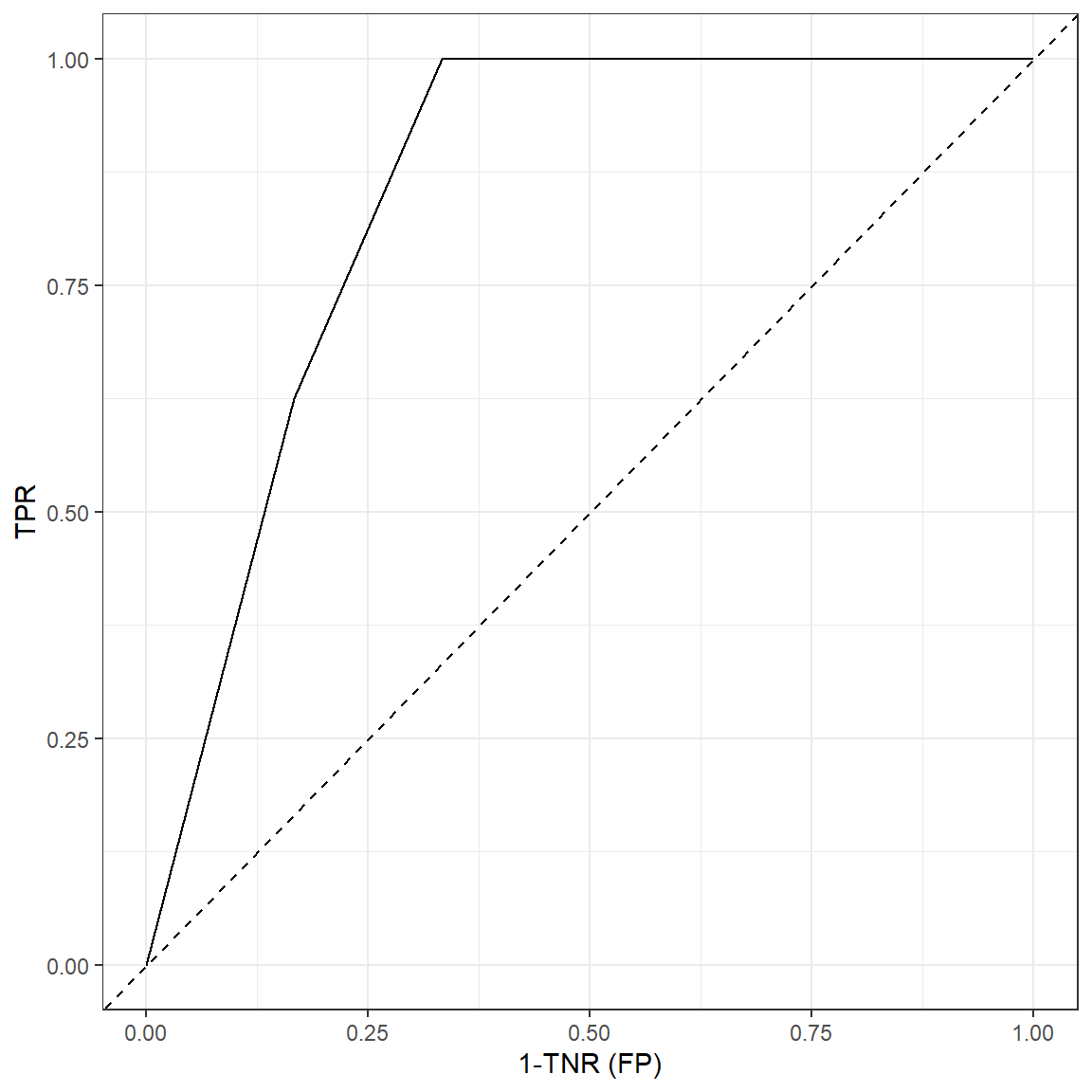

ROC may be a useful plot to inform about model’s predictive power as well as choosing an optimal cut-off value. The area under the ROC curve (AUC or AUROC) is typically used to evaluate the predictive power of classification models. The diagonal line in this plot represents a hypothetical model with no predictive power and AUC for the diagonal line is 0.5 (it is half of the whole square). The more ROC curve resembles with the diagonal line, less the predictive power is. It is not easy to calculate AUC by hand or straight formula as it requires calculus and numerical approximations. There are many alternatives in R to calculate AUC. We will use the cutpointr package as it also provides other tools to select an optimal cut-off point.

# install.packages('cutpointr')

require(cutpointr)

cut.obj <- cutpointr(x     = recidivism_sub$pred_prob,
                     class = recidivism_sub$Recidivism_Arrest_Year2)

plot(cut.obj)

cut.obj$optimal_cutpoint

[1] 0.427855

cut.obj$AUC

[1] 0.8541667

We see that AUC for the predictions in the hypothetical dataset is 0.854. This can be considered as good in terms of predictive power. The closer AUC is to 1, the more predictive power the model has. The closer AUC is to 0.5, the closer predictive power is to random guessing. The magnitude of AUC is also closely related to how well the predicted probabilities are separated for two classes.

The cutpointr package provides more in terms of finding optimal values to maximize certain metrics. For instance, suppose we want to find the optimal cut-off value that maximizes the sum of specificity and sensitivity.

cut.obj <- cutpointr(x      = recidivism_sub$pred_prob,
                     class  = recidivism_sub$Recidivism_Arrest_Year2,
                     method = maximize_metric,
                     metric = sum_sens_spec)

cut.obj$optimal_cutpoint

[1] 0.427855

plot(cut.obj)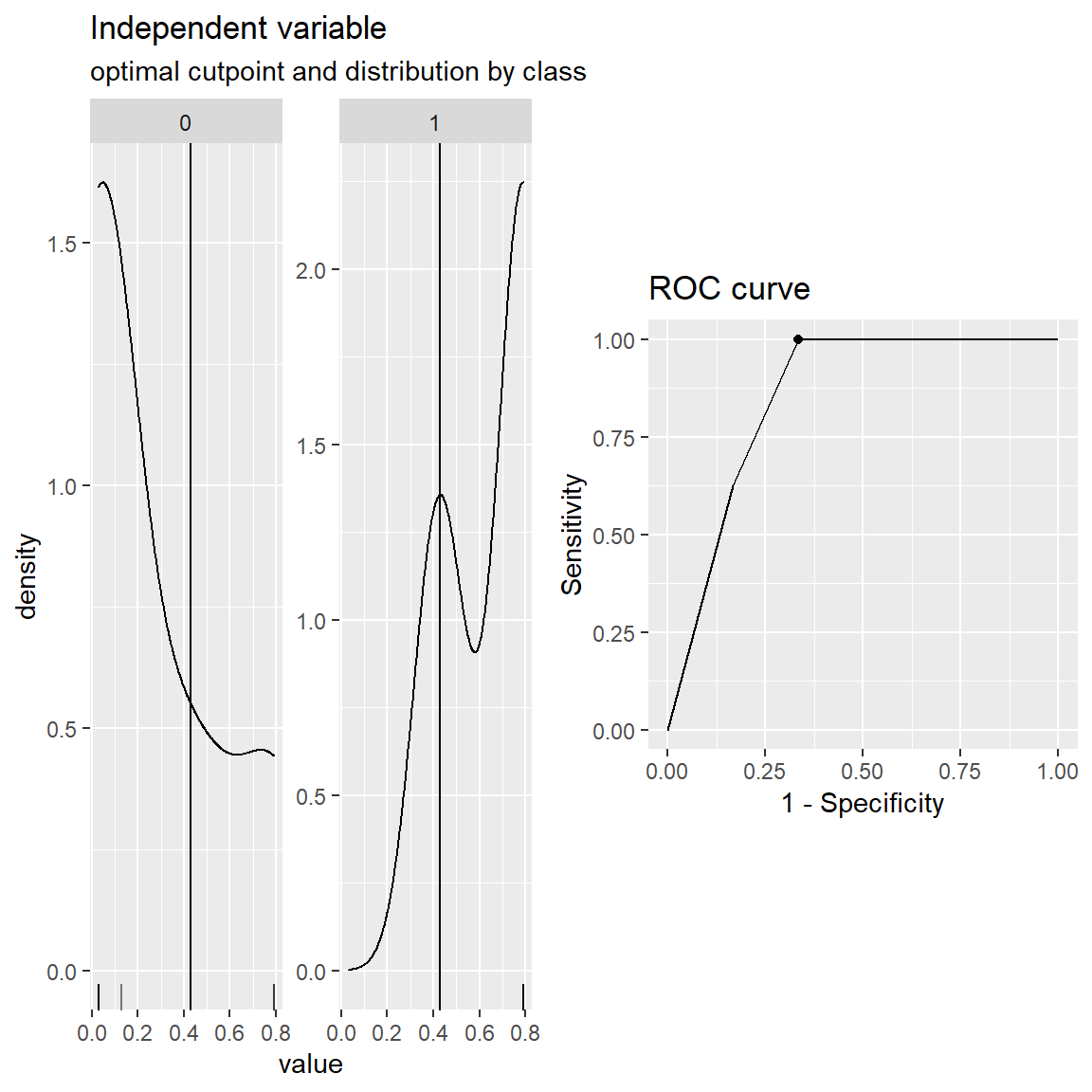

You can also create custom cost functions to maximize if you can attach a $ value to TP, FP, TN, FN. For instance, suppose that a true-positive prediction made by the model brings a 5 dollars profit and a false-positive prediction made by the model costs 1 dollars. A true-negative or a false-negative doesn’t cost or profit anything. Then, you can find an optimal cut-off value that maximizes the total profit.

# Custom function

cost <- function(tp,fp,tn,fn,...){
  my.cost <- matrix(5*tp - 1*fp + 0*tn + 0*fn, ncol = 1)
  colnames(my.cost) <- 'my.cost'
  return(my.cost)
}

cut.obj <- cutpointr(x      = recidivism_sub$pred_prob,
                     class  = recidivism_sub$Recidivism_Arrest_Year2,
                     method = maximize_metric,
                     metric = cost)

cut.obj$optimal_cutpoint

[1] 0.427855

plot(cut.obj)

Check this page to find more information about the cutpointr package.

1.5. Building a Prediction Model for Recidivism using the caret package

Please review the following notebook that builds a classification model using the logistic regression for the full recidivism dataset.

Building a Logistic Regression Model

2. Regularization in Logistic Regression

The regularization works similarly in logistic regression, as discussed in linear regression. We add penalty terms to the loss function to avoid large coefficients, and we reduce model variance by including a penalty term in exchange for adding bias. Optimizing the penalty degree via tuning, we can typically get models with better performance than a logistic regression with no regularization.

2.1 Ridge Penalty

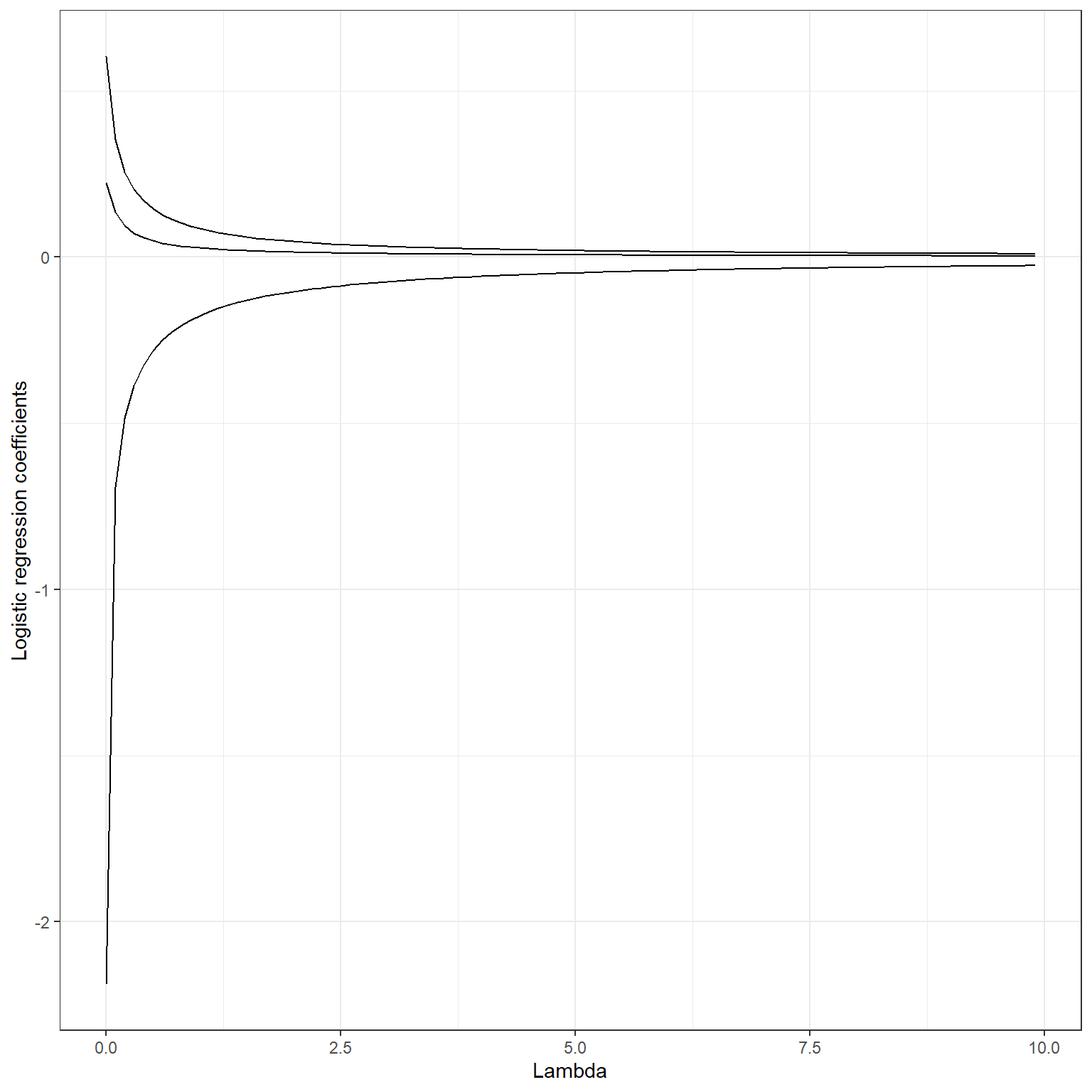
The loss function with ridge penalty applied in logistic regression is the following:

logL(Y|β)=(N∑i=1Yi×ln(Pi)+(1−Yi)×ln(1−Pi))−λ2P∑i=1β2p

Notice that we subtract the penalty from the logistic loss because we maximize the quantity. The penalty term has the same effect in the logistic regression, and it will pull the regression coefficients toward zero but will not make them exactly equal to zero. Below, you can see a plot of change in logistic regression coefficients for some of the variables from a model that will be fit in the next section at increasing levels of ridge penalty.

---

NOTE

The glmnet package divides the value of the loss function by sample size (N) during the optimization (Equation 12 and 2-3 in this paper). It technically does not change anything in terms of the optimal solution. On the other hand, we should be aware that the ridge penalty being applied in the `glmnet package has become

Nλ2P∑i=1β2p.

This information may be necessary while searching plausible values of λ for the glmnet package.

---

Building a Classification Model with Ridge Penalty for Recidivism using the caret package

Please review the following notebook that builds a classification model using the logistic regression with ridge penalty for the full recidivism dataset.

Building a Classification Model with Ridge Penalty

2.2. Lasso Penalty

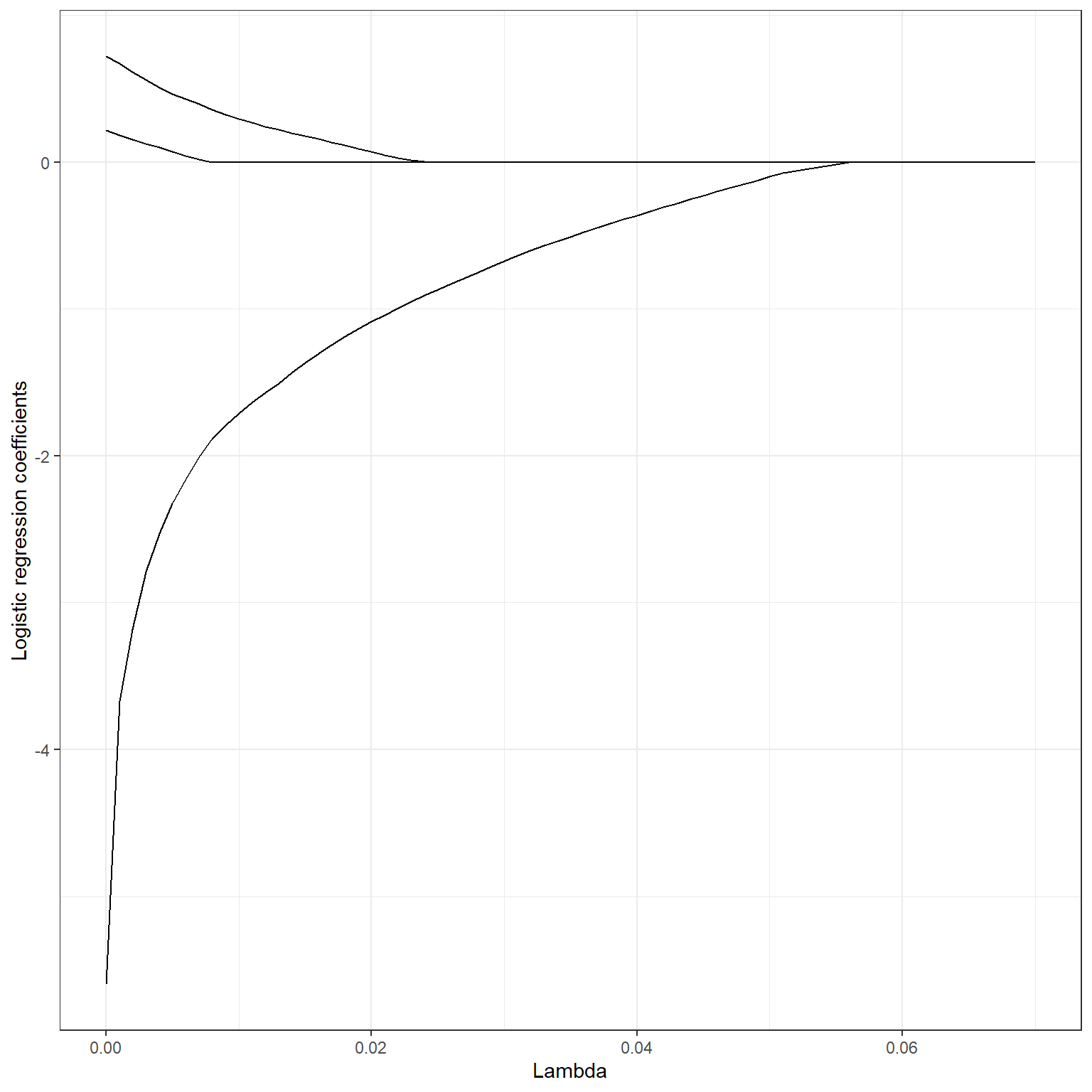
The loss function with the lasso penalty applied in logistic regression is the following: logL(Y|β)=(N∑i=1Yi×ln(Pi)+(1−Yi)×ln(1−Pi))−λP∑i=1|βp|

The penalty term has the same effect in the logistic regression, and it will make the regression coefficients equal to zero when a sufficiently large λ value is applied. Below, you can see a plot of change in logistic regression coefficients for some of the variables from a model that will be fit in the next section at increasing levels of lasso penalty.

---

NOTE

Note that the glmnet package divides the value of the loss function by sample (N) during the optimization (Equation 12 and 2-3 in this paper). You should be aware that the lasso penalty being applied in the `glmnet package has become

NλP∑i=1|βp|.

This information may be important while searching plausible values of λ for the glmnet package.

---

Building a Classification Model with Lasso Penalty for Recidivism using the caret package

Please review the following notebook that builds a classification model using the logistic regression with lasso penalty for the full recidivism dataset.

Building a Classification Model with Lasso Penalty

2.3. Elastic Net

The loss function with the elastic applied is the following:

logL(Y|β)=(N∑i=1Yi×ln(Pi)+(1−Yi)×ln(1−Pi))−((1−α)λ2P∑i=1β2p+αλP∑i=1|βp|)

Building a Classification Model with Elastic Net for Recidivism using the caret package

Please review the following notebook that builds a classification model using the logistic regression with elastic net for the full recidivism dataset.

Building a Classification Model with Elastic Net