[Updated: Sun, Nov 27, 2022 - 14:10:08 ]
1. The Concept of Bootstrap Aggregation (BAGGING)
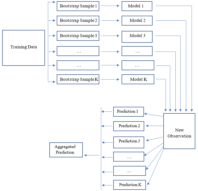
The concept of bagging is based on the idea that predictions from an ensemble of models are better than any single model predictions. Suppose we randomly draw multiple samples from a population and then develop a prediction model for an outcome using each sample. The aggregated predictions from these multiple models would perform better due to the reduced model variance (aggregation would reduce noise due to sampling).
Due to the lack of access to the population (even if we assume there is a well-defined population), we can mimic the sampling from a population by replacing it with bootstrapping. A Bootstrap sample is a random sample with replacement from the sample data.
Suppose there is sample data with ten observations and three predictors. Below are five bootstrap samples from this sample data.
d <- data.frame(x1 =c(20,25,30,42,10,60,65,55,80,90),
                x2 =c(10,15,12,20,45,75,70,80,85,90),
                x3 =c(25,30,35,20,40,80,85,90,92,95),
                label= c('A','B','C','D','E','F','G','H','I','J'))

d
x1 x2 x3 label
1 20 10 25 A
2 25 15 30 B
3 30 12 35 C
4 42 20 20 D
5 10 45 40 E
6 60 75 80 F
7 65 70 85 G
8 55 80 90 H
9 80 85 92 I
10 90 90 95 J x1 x2 x3 label
2 25 15 30 B
2.1 25 15 30 B
6 60 75 80 F
1 20 10 25 A
8 55 80 90 H
10 90 90 95 J
10.1 90 90 95 J
8.1 55 80 90 H
10.2 90 90 95 J
3 30 12 35 C# Bootstrap sample 2
d[sample(1:10,replace = TRUE),] x1 x2 x3 label
4 42 20 20 D
9 80 85 92 I
9.1 80 85 92 I
10 90 90 95 J
6 60 75 80 F
10.1 90 90 95 J
3 30 12 35 C
2 25 15 30 B
9.2 80 85 92 I
4.1 42 20 20 D# Bootstrap sample 3
d[sample(1:10,replace = TRUE),] x1 x2 x3 label
9 80 85 92 I
3 30 12 35 C
6 60 75 80 F
3.1 30 12 35 C
4 42 20 20 D
5 10 45 40 E
4.1 42 20 20 D
8 55 80 90 H
10 90 90 95 J
3.2 30 12 35 C# Bootstrap sample 4
d[sample(1:10,replace = TRUE),] x1 x2 x3 label
8 55 80 90 H
7 65 70 85 G
3 30 12 35 C
1 20 10 25 A
10 90 90 95 J
2 25 15 30 B
9 80 85 92 I
10.1 90 90 95 J
6 60 75 80 F
10.2 90 90 95 J# Bootstrap sample 5
d[sample(1:10,replace = TRUE),] x1 x2 x3 label
3 30 12 35 C
10 90 90 95 J
5 10 45 40 E
8 55 80 90 H
6 60 75 80 F
3.1 30 12 35 C
1 20 10 25 A
4 42 20 20 D
9 80 85 92 I
8.1 55 80 90 HThe process of bagging is building separate models for each bootstrap sample and then applying all these models to a new observation for predicting the outcome. Finally, these predictions are aggregated in some form (e.g., taking the average) to obtain a final prediction for the new observation. The idea of bagging can technically be applied to any prediction model (e.g., CNN’s, regression models). During the model process from each bootstrap sample, no regularization was applied, and models were developed to their full complexity. So, we obtain so many unbiased models. While each model has a significant sample variance, we hope to reduce this sampling variance by aggregating the predictions from all these models at the end.
1.1. BAGGING: Do
It Yourself with the rpart package
In this section, we will apply the bagging idea to decision trees to predict the readability scores. First, we import and prepare data for modeling. Then, we split the data into training and test pieces.
# Import the dataset

readability <- read.csv(here('data/readability_features.csv'),header=TRUE)

# Write the recipe

require(recipes)

blueprint_readability <- recipe(x     = readability,
                    vars  = colnames(readability),
                    roles = c(rep('predictor',768),'outcome')) %>%
             step_zv(all_numeric()) %>%
             step_nzv(all_numeric()) %>%
             step_normalize(all_numeric_predictors())

# Train/Test Split

set.seed(10152021)  # for reproducibility

loc      <- sample(1:nrow(readability), round(nrow(readability) * 0.9))
read_tr  <- readability[loc, ]
read_te  <- readability[-loc, ]

dim(read_tr)

dim(read_te)
The code below will take a
- bootstrap sample from training data,
- develop a full tree model with no pruning, and
- save the model object as an element of a list.
We will repeat this process ten times.
require(caret)

bag.models <- vector('list',10)

for(i in 1:10){

  # Bootstrap sample

    temp_rows <- sample(1:nrow(read_tr),nrow(read_tr),replace=TRUE)

    temp <- read_tr[temp_rows,]

  # Train the tree model with no pruning and no cross validation

    grid <- data.frame(cp=0)
    cv <- trainControl(method = "none")

    bag.models[[i]] <- caret::train(blueprint_readability,
                                    data      = temp,
                                    method    = 'rpart',
                                    tuneGrid  = grid,
                                    trControl = cv,
                                    control   = list(minsplit=20,
                                                     minbucket = 2,
                                                     maxdepth = 60))

}
Now, we will use each of these models to predict the readability score for the test data. We will also average these predictions. Then, we will save the predictions in a matrix form to compare.
preds <- data.frame(obs = read_te[,c('target')])

preds$model1  <- predict(bag.models[[1]],read_te)
preds$model2  <- predict(bag.models[[2]],read_te)
preds$model3  <- predict(bag.models[[3]],read_te)
preds$model4  <- predict(bag.models[[4]],read_te)
preds$model5  <- predict(bag.models[[5]],read_te)
preds$model6  <- predict(bag.models[[6]],read_te)
preds$model7  <- predict(bag.models[[7]],read_te)
preds$model8  <- predict(bag.models[[8]],read_te)
preds$model9  <- predict(bag.models[[9]],read_te)
preds$model10 <- predict(bag.models[[10]],read_te)

preds$average <- rowMeans(preds[,2:11])

head(round(preds,3))
obs model1 model2 model3 model4 model5 model6 model7 model8
1 0.246 -0.827 0.355 0.619 -0.925 -0.956 0.260 -0.095 -0.224
2 -0.188 -1.399 -0.963 -0.458 0.635 -0.415 -0.684 -0.101 -0.963
3 -0.135 -0.235 1.149 0.827 0.663 0.015 0.865 0.693 -0.013
4 0.395 0.690 0.355 1.361 0.025 -0.271 0.119 -0.406 -0.044
5 -0.371 -1.232 -0.901 -1.968 -1.147 -1.420 -1.393 -1.104 0.114
6 -1.156 -0.173 -0.531 -0.694 -1.390 -0.508 -0.690 -0.769 0.360
model9 model10 average
1 -0.610 0.433 -0.197
2 -0.610 0.259 -0.470
3 0.242 -0.253 0.395
4 0.005 0.739 0.257
5 -1.024 -1.125 -1.120
6 -0.252 -0.894 -0.554Now, let’s compute the RMSE for each model’s predicted scores and the RMSE for the average of predicted scores from all ten tree models.
p1 <- sqrt(mean((preds$obs - preds$model1)^2))
p2 <- sqrt(mean((preds$obs - preds$model2)^2))
p3 <- sqrt(mean((preds$obs - preds$model3)^2))
p4 <- sqrt(mean((preds$obs - preds$model4)^2))
p5 <- sqrt(mean((preds$obs - preds$model5)^2))
p6 <- sqrt(mean((preds$obs - preds$model6)^2))
p7 <- sqrt(mean((preds$obs - preds$model7)^2))
p8 <- sqrt(mean((preds$obs - preds$model8)^2))
p9 <- sqrt(mean((preds$obs - preds$model9)^2))
p10 <- sqrt(mean((preds$obs - preds$model10)^2))

p.ave <- sqrt(mean((preds$obs - preds$average)^2))


ggplot()+
  geom_point(aes(x = 1:11,y=c(p1,p2,p3,p4,p5,p6,p7,p8,p9,p10,p.ave)))+
  xlab('Model Predictions') +
  ylab('RMSE') +
  ylim(0,1) +
  scale_x_continuous(breaks = 1:11,
                     labels=c('Model 1','Model 2', 'Model 3', 'Model 4',
                              'Model 5','Model 6', 'Model 7', 'Model 8',
                              'Model 9','Model 10','Bagged'))+
  theme_bw()+
  annotate('text',
           x = 1:11,
           y=c(p1,p2,p3,p4,p5,p6,p7,p8,p9,p10,p.ave)*1.03,
           label = round(c(p1,p2,p3,p4,p5,p6,p7,p8,p9,p10,p.ave),3),
           cex=3)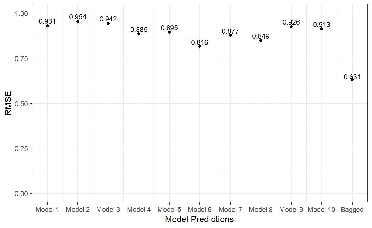
As it is evident, the bagging of 10 different tree models significantly improved the predictions on the test dataset.
1.2. BAGGING
with the ranger and caret::train()
packages
Instead of writing your code to implement the idea of bagging for
decision trees, we can use the ranger method via
caret::train().
require(ranger)

getModelInfo()$ranger$parameters
parameter class label
1 mtry numeric #Randomly Selected Predictors
2 splitrule character Splitting Rule
3 min.node.size numeric Minimal Node SizeThe caret::train() allows us manipulate three parameters
while using the ranger method:
splitrule: set this to ‘variance’ for regression problems with continuous outcome. Other alternatives are
extratrees,maxstat, andbeta.min.node.size.: this is identical to
minbucketargument in therpartmethod and indicates the minimum number of observations for each node.mtry: this is the most critical parameter for this method and indicates the number of predictors to consider for developing tree models. For bagged decision trees, you can set this to the number of all predictors in your model
# Cross validation settings

    read_tr = read_tr[sample(nrow(read_tr)),]

    # Create 10 folds with equal size

    folds = cut(seq(1,nrow(read_tr)),breaks=10,labels=FALSE)

    # Create the list for each fold

    my.indices <- vector('list',10)
    for(i in 1:10){
      my.indices[[i]] <- which(folds!=i)
    }

    cv <- trainControl(method = "cv",
                       index  = my.indices)

# Grid, running with all predictors in the data (768)

grid <- expand.grid(mtry = 768,splitrule='variance',min.node.size=2)
grid
mtry splitrule min.node.size
1 768 variance 2# Bagging with 10 tree models
bagged.trees <- caret::train(blueprint_readability,
data = read_tr,
method = 'ranger',
trControl = cv,
tuneGrid = grid,
num.trees = 10,
max.depth = 60)Let’s check the cross-validated performance metrics.
bagged.trees$results mtry splitrule min.node.size RMSE Rsquared MAE
1 768 variance 2 0.6804536 0.5683141 0.543069
RMSESD RsquaredSD MAESD
1 0.02011178 0.02586802 0.01373682The performance is very similar to what we got in our DIY demonstration.
A couple of things to note:
When you set
max.depth=argument within thecaret::trainfunction, it passes this to therangerfunction. Try to set this number to as large as possible, so you develop each tree to its full capacity.The penalty term is technically zero (
cpparameter in therpartfunction) while building each tree model. In Bagging, we deal with the model variance differently. Instead of applying a penalty term, we ensemble many unpenalized tree models to reduce the model variance.It is a little tricky to obtain reproducible results from this procedure. See this link to learn more about accomplishing that.
The number of trees (bootstrap samples) is a hyperparameter to tune. Conceptually, the model performance will improve as you increase the number of tree models used in Bagging; however, the performance will stabilize at some point. It is a tuning process to find the minimum number of tree models in Bagging to obtain the maximal model performance.
1.3. Tuning the Number of Tree Models in Bagging
Unfortunately, caret::train does not let us define the
num.trees argument as a hyperparameter in the grid search.
So, the only way to search for the optimal number of trees is to use the
ranger method via caret::train function and
iterate over a set of values for the num.trees argument.
Then, compare the model performance and pick the optimal number of tree
models.
The code below implements this idea and saves the results from each iteration in a list object.
# Run the bagged trees by iterating over num.trees using the
# values 5, 20, 40, 60,  ..., 200

  nbags <- c(5,seq(from = 20,to = 200, by = 20))

  bags <- vector('list',length(nbags))

    for(i in 1:length(nbags)){

      bags[[i]] <- caret::train(blueprint_readability,
                                data      = read_tr,
                                method    = 'ranger',
                                trControl = cv,
                                tuneGrid  = grid,
                                num.trees = nbags[i],
                                max.depth = 60)

      print(i)

    }

    # This can take a few hours to run.
Let’s check the cross-validated RMSE for the bagged tree models with different number of trees.
rmses <- c()

for(i in 1:length(nbags)){

  rmses[i] = bags[[i]]$results$RMSE

}

ggplot()+
  geom_line(aes(x=nbags,y=rmses))+
  xlab('Number of Trees')+
  ylab('RMSE')+
  ylim(c(0.6,0.75))+
  theme_bw()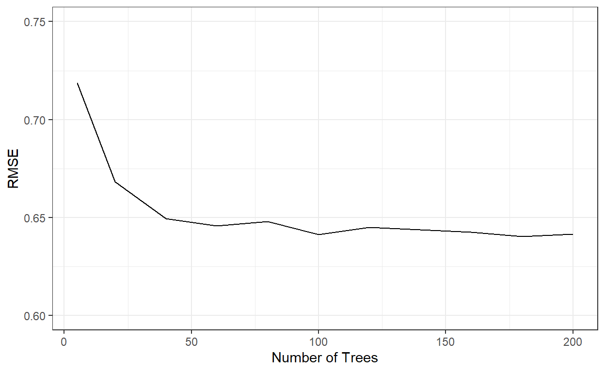
nbags[which.min(rmses)][1] 180It indicates that the RMSE stabilizes after roughly 60 tree models. We can see that a bagged tree model with 180 trees gave the best result. Let’s see how well this model performs on the test data.
# Predictions from a Bagged tree model with 180 trees

predicted_te <- predict(bags[[10]],read_te)

# MAE

mean(abs(read_te$target - predicted_te))
[1] 0.4776075[1] 0.6003086# R-square
cor(read_te$target,predicted_te)^2[1] 0.6646118Now, we can add this to our comparison list to remember how well this performs compared to other methods.
| R-square | MAE | RMSE | |
|---|---|---|---|
| Linear Regression | 0.658 | 0.499 | 0.620 |
| Ridge Regression | 0.727 | 0.432 | 0.536 |
| Lasso Regression | 0.721 | 0.433 | 0.542 |
| Elastic Net | 0.726 | 0.433 | 0.539 |
| KNN | 0.611 | 0.519 | 0.648 |
| Decision Tree | 0.499 | 0.574 | 0.724 |
| Bagged Trees | 0.664 | 0.478 | 0.600 |
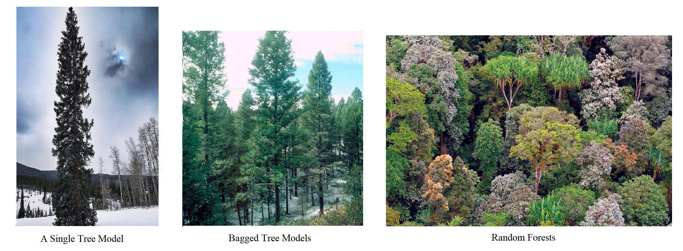
2. Random Forests
Random Forests is an idea very similar to Bagging with an extra feature. In Random Forests, while we take a bootstrap sample of observations (a random sample of rows in training data with replacement), we also take a random sample of columns for each split while developing a tree model. It allows us to develop tree models more independently of each other.
When specific important predictors are related to the outcome, the tree models developed using all predictors will be very similar, particularly at the top nodes, although we take bootstrap samples. These trees will be correlated to each other, which may reduce the efficiency of BAGGING in reducing the variance. We can diversify the tree models by randomly sampling a certain number of predictors while developing each tree. It turns out that a diverse group of tree models does much better in predicting the outcome than a group of tree models similar to each other.
We can use the same ranger package to fit the random
forests models by only changing the mtry argument in our
grid. Below, we will fit a random forests model with ten trees by
randomly sampling from rows for each tree. In addition, when we develop
each tree model, we will also randomly sample 300 predictors. I set
mtry=300 in the grid object, indicating that
it will randomly sample 300 predictors to consider for each split when
developing each tree.
# Grid, randomly sample 300 predictors

grid <- expand.grid(mtry = 300,splitrule='variance',min.node.size=2)
grid
mtry splitrule min.node.size
1 300 variance 2# Random Forest with 10 tree models
rforest <- caret::train(blueprint_readability,
data = read_tr,
method = 'ranger',
trControl = cv,
tuneGrid = grid,
num.trees = 10,
max.depth = 60)
rforest$times$everything
user system elapsed
177.76 1.08 133.97
$final
user system elapsed
15.87 0.05 11.38
$prediction
[1] NA NA NALet’s check the cross-validated performance metrics.
rforest$results mtry splitrule min.node.size RMSE Rsquared MAE
1 300 variance 2 0.6829234 0.5674509 0.5430574
RMSESD RsquaredSD MAESD
1 0.01628784 0.02833995 0.01213438For random forests, there are two hyperparameters to tune:
mtry, the number of predictors to choose for each split during the tree model developmentnum.trees, the number of trees.
As mentioned before, unfortunately, the caret::train
only allows mtry in the grid search. For the number of
trees, one should embed it in a for loop to iterate over a
set of values. The code below hypothetically implements this idea by
trying ten different mtry values
(100,150,200,250,300,350,400,450,500,550) and saves the results from
each iteration in a list object. However, I haven’t run it, which may
take a long time.
# Grid Settings

    grid <- expand.grid(mtry = c(100,150,200,250,300,350,400,450,500,550),
                        splitrule='variance',
                        min.node.size=2)

# Run the bagged trees by iterating over num.trees values from 1 to 200

    bags <- vector('list',200)

    for(i in 1:200){

      bags[[i]] <- caret::train(blueprint_readability,
                                data      = read_tr,
                                method    = 'ranger',
                                trControl = cv,
                                tuneGrid  = grid,
                                num.trees = i,
                                max.depth = 60,)

    }
Instead, I run this by fixing mtry=300 and then
iterating over the number of trees for values of 5, 20, 40, 60, 80, …,
200 (as we did for bagged trees).
rmses <- c()

for(i in 1:length(nbags)){

  rmses[i] = bags[[i]]$results$RMSE

}

ggplot()+
  geom_line(aes(x=nbags,y=rmses))+
  xlab('Number of Trees')+
  ylab('RMSE')+
  ylim(c(0.6,0.75))+
  theme_bw()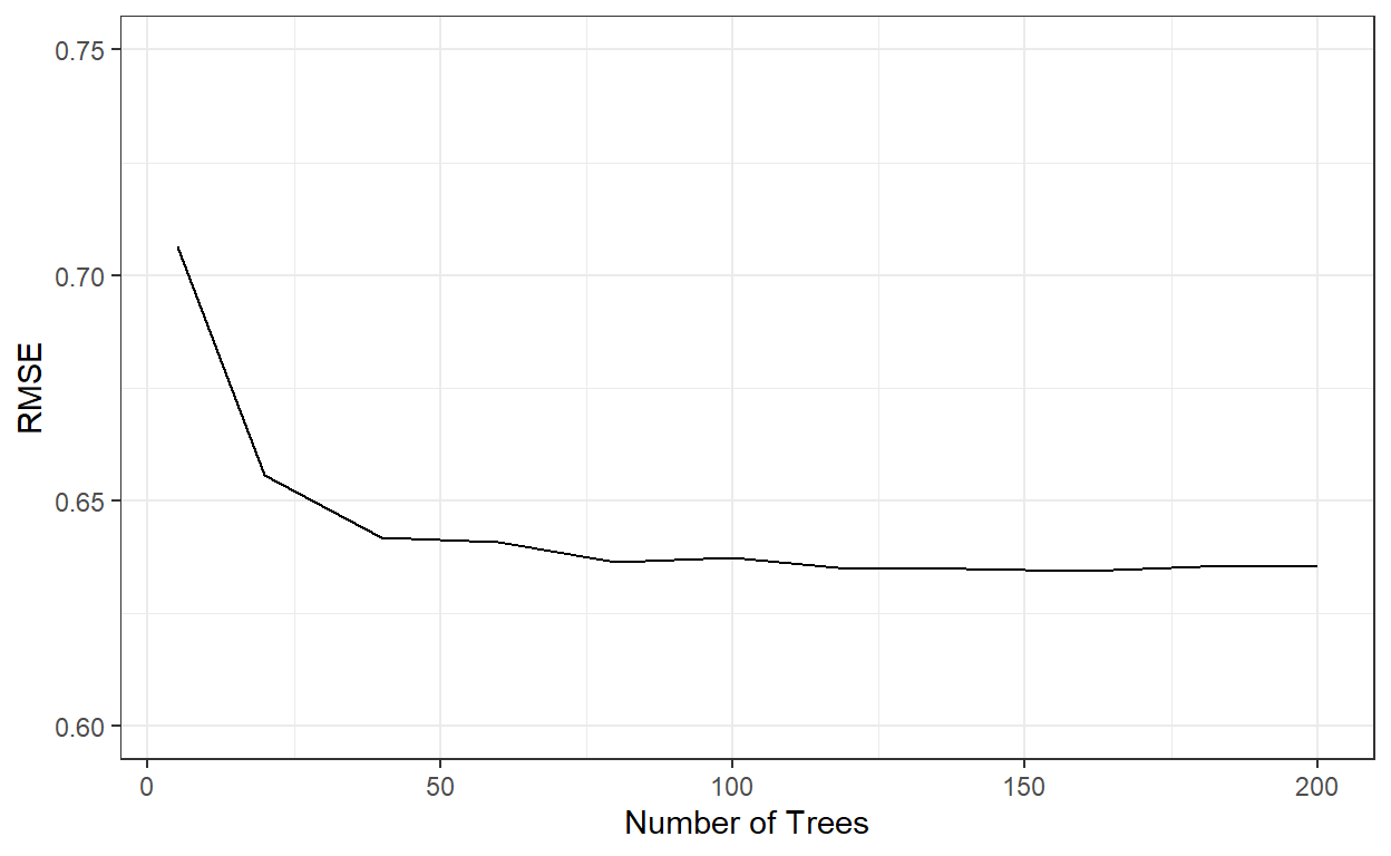
nbags[which.min(rmses)][1] 160RMSE similarly stabilized after roughly 60 trees. Let’s see how well the model with 200 trees perform.
# Predictions from a Random Forest model with 160 trees

predicted_te <- predict(bags[[11]],read_te)

# MAE

mean(abs(read_te$target - predicted_te))
[1] 0.4756419[1] 0.6003527# R-square
cor(read_te$target,predicted_te)^2[1] 0.6690829Below is our comparison table with Random Forests added. As you see,
there is a slight improvement over Bagged Trees, and we can improve this
a little more by trying different values of mtry and
finding an optimal number.
| R-square | MAE | RMSE | |
|---|---|---|---|
| Linear Regression | 0.658 | 0.499 | 0.620 |
| Ridge Regression | 0.727 | 0.432 | 0.536 |
| Lasso Regression | 0.721 | 0.433 | 0.542 |
| Elastic Net | 0.726 | 0.433 | 0.539 |
| KNN | 0.611 | 0.519 | 0.648 |
| Decision Tree | 0.499 | 0.574 | 0.724 |
| Bagged Trees | 0.664 | 0.478 | 0.600 |
| Random Forests | 0.669 | 0.476 | 0.600 |
3. Predicting Recidivism using Bagges Trees and Random Forests
In this section, I provide the R code to predict recidivism using Bagged Trees and Random Forests.
Import the recidivism dataset and pre-process the variables
# Import data

recidivism <- read.csv('./data/recidivism_y1 removed and recoded.csv',header=TRUE)

# Write the recipe

  # List of variable types

  outcome <- c('Recidivism_Arrest_Year2')

  id      <- c('ID')

  categorical <- c('Residence_PUMA',
                   'Prison_Offense',
                   'Age_at_Release',
                   'Supervision_Level_First',
                   'Education_Level',
                   'Prison_Years',
                   'Gender',
                   'Race',
                   'Gang_Affiliated',
                   'Prior_Arrest_Episodes_DVCharges',
                   'Prior_Arrest_Episodes_GunCharges',
                   'Prior_Conviction_Episodes_Viol',
                   'Prior_Conviction_Episodes_PPViolationCharges',
                   'Prior_Conviction_Episodes_DomesticViolenceCharges',
                   'Prior_Conviction_Episodes_GunCharges',
                   'Prior_Revocations_Parole',
                   'Prior_Revocations_Probation',
                   'Condition_MH_SA',
                   'Condition_Cog_Ed',
                   'Condition_Other',
                   'Violations_ElectronicMonitoring',
                   'Violations_Instruction',
                   'Violations_FailToReport',
                   'Violations_MoveWithoutPermission',
                   'Employment_Exempt')

  numeric   <- c('Supervision_Risk_Score_First',
                 'Dependents',
                 'Prior_Arrest_Episodes_Felony',
                 'Prior_Arrest_Episodes_Misd',
                 'Prior_Arrest_Episodes_Violent',
                 'Prior_Arrest_Episodes_Property',
                 'Prior_Arrest_Episodes_Drug',
                 'Prior_Arrest_Episodes_PPViolationCharges',
                 'Prior_Conviction_Episodes_Felony',
                 'Prior_Conviction_Episodes_Misd',
                 'Prior_Conviction_Episodes_Prop',
                 'Prior_Conviction_Episodes_Drug',
                 'Delinquency_Reports',
                 'Program_Attendances',
                 'Program_UnexcusedAbsences',
                 'Residence_Changes',
                 'Avg_Days_per_DrugTest',
                 'Jobs_Per_Year')

  props      <- c('DrugTests_THC_Positive',
                  'DrugTests_Cocaine_Positive',
                  'DrugTests_Meth_Positive',
                  'DrugTests_Other_Positive',
                  'Percent_Days_Employed')

  # Convert all nominal, ordinal, and binary variables to factors

  for(i in categorical){

    recidivism[,i] <- as.factor(recidivism[,i])

  }

  # Blueprint for processing variables

  require(recipes)

  blueprint_recidivism <- recipe(x  = recidivism,
                      vars  = c(categorical,numeric,props,outcome,id),
                      roles = c(rep('predictor',48),'outcome','ID')) %>%
    step_indicate_na(all_of(categorical),all_of(numeric),all_of(props)) %>%
    step_zv(all_numeric()) %>%
    step_impute_mean(all_of(numeric),all_of(props)) %>%
    step_impute_mode(all_of(categorical)) %>%
    step_logit(all_of(props),offset=.001) %>%
    step_poly(all_of(numeric),all_of(props),degree=2) %>%
    step_normalize(paste0(numeric,'_poly_1'),
                   paste0(numeric,'_poly_2'),
                   paste0(props,'_poly_1'),
                   paste0(props,'_poly_2')) %>%
    step_dummy(all_of(categorical),one_hot=TRUE) %>%
    step_num2factor(Recidivism_Arrest_Year2,
                    transform = function(x) x + 1,
                    levels=c('No','Yes'))

  blueprint_recidivism
2. Train/Test Split
  loc <- which(recidivism$Training_Sample==1)

  # Training dataset

  recidivism_tr  <- recidivism[loc, ]
  dim(recidivism_tr)

  # Test dataset

  recidivism_te  <- recidivism[-loc, ]
  dim(recidivism_te)
3.1. Bagged Trees
# Cross validation settings

    set.seed(10302021) # for reproducibility

    recidivism_tr = recidivism_tr[sample(nrow(recidivism_tr)),]

  # Create 10 folds with equal size

    folds = cut(seq(1,nrow(recidivism_tr)),breaks=10,labels=FALSE)

  # Create the list for each fold

    my.indices <- vector('list',10)
    for(i in 1:10){
      my.indices[[i]] <- which(folds!=i)
    }


  cv <- trainControl(method = "cv",
                     index  = my.indices,
                     classProbs = TRUE,
                     summaryFunction = mnLogLoss)

# Grid settings

  # Notice that I use **'gini'** for splitrule because this is
  # now a classification problem.

  grid <- expand.grid(mtry = 142,
                    splitrule='gini',
                    min.node.size=2)
  grid

# Run the BAGGED Trees with different number of trees
# 5, 20, 40, 60, ..., 200

    nbags <- c(5,seq(20,200,20))

    bags <- vector('list',length(nbags))

    for(i in 1:length(nbags)){

      bags[[i]] <- caret::train(blueprint_recidivism,
                                data      = recidivism_tr,
                                method    = 'ranger',
                                trControl = cv,
                                tuneGrid  = grid,
                                metric    = 'logLoss',
                                num.trees = nbags[i],
                                max.depth = 60)
    }
logLoss_ <- c()
for(i in 1:length(nbags)){
logLoss_[i] = bags[[i]]$results$logLoss
}
ggplot()+
geom_line(aes(x=nbags,y=logLoss_))+
xlab('Number ofs')+
ylab('Negative LogLoss')+
ylim(c(0.4,2))+
theme_bw()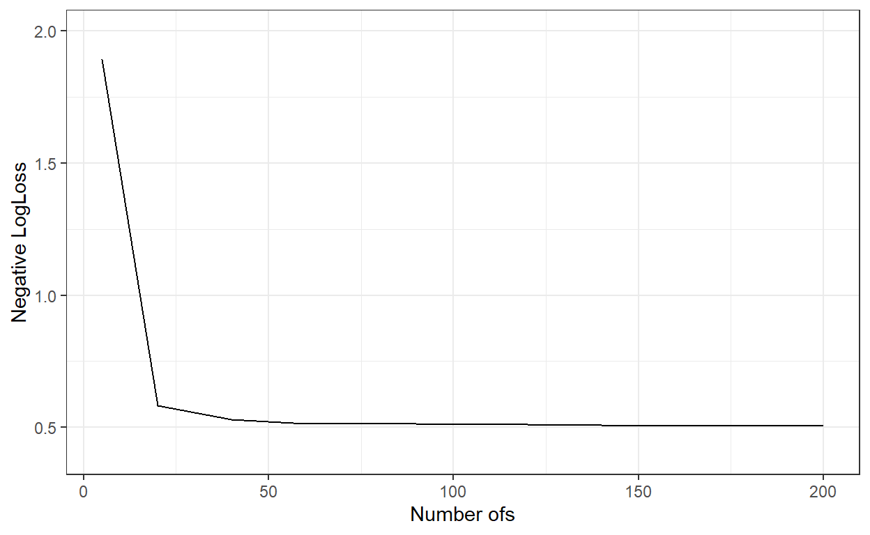
nbags[which.min(logLoss_)][1] 200# Predict the probabilities for the observations in the test dataset
predicted_te <- predict(bags[[11]], recidivism_te, type='prob')
dim(predicted_te)[1] 5460 2head(predicted_te) No Yes
1 0.9900 0.0100
2 0.6050 0.3950
3 0.6150 0.3850
4 0.5675 0.4325
5 0.7725 0.2275
6 0.6900 0.3100# Compute the AUC
require(cutpointr)
cut.obj <- cutpointr(x = predicted_te$Yes,
class = recidivism_te$Recidivism_Arrest_Year2)
auc(cut.obj)[1] 0.7241845# Confusion matrix assuming the threshold is 0.5
pred_class <- ifelse(predicted_te$Yes>.5,1,0)
confusion <- table(recidivism_te$Recidivism_Arrest_Year2,pred_class)
confusion pred_class
0 1
0 3957 189
1 1125 189# True Negative Rate
confusion[1,1]/(confusion[1,1]+confusion[1,2])[1] 0.9544139# False Positive Rate
confusion[1,2]/(confusion[1,1]+confusion[1,2])[1] 0.04558611# True Positive Rate
confusion[2,2]/(confusion[2,1]+confusion[2,2])[1] 0.1438356# Precision
confusion[2,2]/(confusion[1,2]+confusion[2,2])[1] 0.5| -LL | AUC | ACC | TPR | TNR | FPR | PRE | |
|---|---|---|---|---|---|---|---|
| Bagged Trees | 0.506 | 0.724 | 0.759 | 0.144 | 0.954 | 0.046 | 0.500 |
| Logistic Regression | 0.510 | 0.719 | 0.755 | 0.142 | 0.949 | 0.051 | 0.471 |
| Logistic Regression with Ridge Penalty | 0.511 | 0.718 | 0.754 | 0.123 | 0.954 | 0.046 | 0.461 |
| Logistic Regression with Lasso Penalty | 0.509 | 0.720 | 0.754 | 0.127 | 0.952 | 0.048 | 0.458 |
| Logistic Regression with Elastic Net | 0.509 | 0.720 | 0.753 | 0.127 | 0.952 | 0.048 | 0.456 |
| KNN | ? | ? | ? | ? | ? | ? | ? |
| Decision Tree | 0.558 | 0.603 | 0.757 | 0.031 | 0.986 | 0.014 | 0.423 |
3.2. Random Forests
# Grid settings

grid <- expand.grid(mtry = 80,splitrule='gini',min.node.size=2)

    # The only difference for random forests is that I set mtry = 80

# Run the Random Forests with different number of trees
# 5, 20, 40, 60, ..., 200

   nbags <- c(5,seq(20,200,20))
   bags <- vector('list',length(nbags))

    for(i in 1:length(nbags)){

      bags[[i]] <- caret::train(blueprint_recidivism,
                                data      = recidivism_tr,
                                method    = 'ranger',
                                trControl = cv,
                                tuneGrid  = grid,
                                metric    = 'logLoss',
                                num.trees = nbags[i],
                                max.depth = 60)
    }
logLoss_ <- c()
for(i in 1:length(nbags)){
logLoss_[i] = bags[[i]]$results$logLoss
}
ggplot()+
geom_line(aes(x=nbags,y=logLoss_))+
xlab('Number ofs')+
ylab('Negative LogLoss')+
ylim(c(0.4,2))+
theme_bw()
nbags[which.min(logLoss_)][1] 180# Predict the probabilities for the observations in the test dataset
predicted_te <- predict(bags[[10]], recidivism_te, type='prob')
# Compute the AUC
cut.obj <- cutpointr(x = predicted_te$Yes,
class = recidivism_te$Recidivism_Arrest_Year2)
auc(cut.obj)[1] 0.7251904# Confusion matrix assuming the threshold is 0.5
pred_class <- ifelse(predicted_te$Yes>.5,1,0)
confusion <- table(recidivism_te$Recidivism_Arrest_Year2,pred_class)
confusion pred_class
0 1
0 3956 190
1 1113 201# True Negative Rate
confusion[1,1]/(confusion[1,1]+confusion[1,2])[1] 0.9541727# False Positive Rate
confusion[1,2]/(confusion[1,1]+confusion[1,2])[1] 0.0458273# True Positive Rate
confusion[2,2]/(confusion[2,1]+confusion[2,2])[1] 0.152968# Precision
confusion[2,2]/(confusion[1,2]+confusion[2,2])[1] 0.5140665| -LL | AUC | ACC | TPR | TNR | FPR | PRE | |
|---|---|---|---|---|---|---|---|
| Random Forests | 0.507 | 0.725 | 0.761 | 0.153 | 0.954 | 0.046 | 0.514 |
| Bagged Trees | 0.506 | 0.724 | 0.759 | 0.144 | 0.954 | 0.046 | 0.500 |
| Logistic Regression | 0.510 | 0.719 | 0.755 | 0.142 | 0.949 | 0.051 | 0.471 |
| Logistic Regression with Ridge Penalty | 0.511 | 0.718 | 0.754 | 0.123 | 0.954 | 0.046 | 0.461 |
| Logistic Regression with Lasso Penalty | 0.509 | 0.720 | 0.754 | 0.127 | 0.952 | 0.048 | 0.458 |
| Logistic Regression with Elastic Net | 0.509 | 0.720 | 0.753 | 0.127 | 0.952 | 0.048 | 0.456 |
| KNN | ? | ? | ? | ? | ? | ? | ? |
| Decision Tree | 0.558 | 0.603 | 0.757 | 0.031 | 0.986 | 0.014 | 0.423 |